A SIMPLE MODEL OF THE CONVECTIVE INTERNAL BOUNDARY LAYER AND ITS APPLICATION TO SURFACE HEAT FLUX ESTIMATES WITHIN POLYNYAS IAN A. RENFREW? and JOHN C. KING British Antarctic Survey, Cambridge, U.K.
(Received in final form 28 September 1999)
Abstract. A simple model of the convective (thermal) internal boundary layer has been developed for climatological studies of air-sea-ice interaction, where in situ observations are scarce and firstorder estimates of surface heat fluxes are required. It is a mixed-layer slab model, based on a steadystate solution of the conservation of potential temperature equation, assuming a balance between advection and turbulent heat-flux convergence. Both the potential temperature and the surface heat flux are allowed to vary with fetch, so the subsequent boundary-layer modification alters the flux convergence and thus the boundary-layer growth rate. For simplicity, microphysical and radiative processes are neglected. The model is validated using several case studies. For a clear-sky cold-air outbreak over a coastal polynya the observed boundary-layer heights, mixed-layer potential temperatures and surface heat fluxes are all well reproduced. In other cases, where clouds are present, the model still captures most of the observed boundary-layer modification, although there are increasing discrepancies with fetch, due to the neglected microphysical and radiative processes. The application of the model to climatological studies of air-sea interaction within coastal polynyas is discussed. Keywords: Cold-air outbreak, Surface heat fluxes, Polynyas, Ronne Ice Shelf, Thermal internal boundary layer.
1. Introduction A convective internal boundary layer generally develops in two archetypal atmospheric flows. The first is when relatively cold maritime air is advected over a warm land surface, whereupon a positive surface sensible heat flux into the boundary layer triggers convection and leads to a deepening of the mixed layer. The second is when relatively cold continental air is advected over a warm ocean or lake, and again a positive surface sensible heat flux triggers convection and boundary-layer deepening (Figure 1). The boundary-layer that develops is termed a thermal internal boundary layer, as it arises primarily from a discontinuity in surface temperature (e.g., Garratt, 1990). To emphasise that convective mixing is taking place we shall use the abbreviation CIBL to mean a convective (thermal) internal boundary layer, following Hsu (1984) and Chang and Braham (1991). ? Author for correspondence: British Antarctic Survey, High Cross, Madingley Road, Cambridge,
CB3 0ET, UK. E-mail:
[email protected] Boundary-Layer Meteorology 94: 335–356, 2000. © 2000 Kluwer Academic Publishers. Printed in the Netherlands.
336
IAN A. RENFREW AND JOHN C. KING
Figure 1. A sketch of a convective (thermal) internal boundary layer development for a cold air outbreak over relatively warm water. The model developed here can be used to predict the CIBL height h(x), mixed-layer potential temperature θm (x), and surface sensible heat flux Hs (x) from upstream surface data, given an initial height h0 , and an ambient stability γθ .
The first scenario, that of daytime CIBL growth over land, has received a fair degree of research attention, as interest has been motivated by concerns over the downward mixing of pollution from chimney stacks. During onshore flow, a chimney stack located on the coast would have its exhaust plume advected downstream, and at some point it will intercept the growing coastal CIBL. Here a downward mixing of the plume by the convective turbulence in the mixed layer leads to localised pollution at the surface, clearly a potentially serious health and environmental concern. Of the models developed to examine this situation, a number of very simple ones appear to reproduce CIBL height observations well and compare favourably to more complete boundary-layer models (e.g., Venkatram, 1977; Gamo et al., 1983; Stunder and SethuRaman, 1985), although Venkatram (1986) points out that the usefulness of these simple models is limited by the data set used to tune the model parameters. The simple models often take the form h = Cx 1/2 , where h is the CIBL height, x is fetch, and C is a constant, typically dependent upon upstream stratification, mixed-layer wind speed, the surface heat flux, and sometimes entrainment at the CIBL top. The second scenario, that of relatively cold continental air flowing over a warm ocean or lake, is somewhat more complicated as the ensuing boundary layer will tend to be moist and cloud filled. Hence microphysical and radiative processes will be important. A number of modelling studies have addressed this scenario with models of varying complexity, for example, Stage and Businger (1981), Hsu (1984), Boers et al. (1990), Pinto et al. (1995), and Flamant and Pelon (1996). These models were generally developed to examine particular CIBL case studies
A SIMPLE MODEL OF THE CONVECTIVE INTERNAL BOUNDARY LAYER
337
and so were tailored to those cases. The model developed here will be used for climatological studies of air-sea interaction over high latitude oceans, and in particular to allow estimates of heat exchange within coastal polynyas. Hence it would be advantageous if our model was simple, and focussed on the changes in surface heat flux with fetch, rather than on accurate prediction of the CIBL height. Coastal polynyas around the Antarctic are typically 5–50 km wide (Smith et al., 1990; Markus et al., 1998), so the model should be appropriate for this scale. Over such distances, a certain amount of boundary-layer modification occurs, most notably a warming and moistening of the CIBL with fetch, due primarily to heat and moisture flux convergence (e.g., Grossman and Betts, 1990; Chang and Braham, 1991; Brümmer, 1997; Renfrew and Moore, 1999). This leads to a decrease in the surface heat flux with fetch, given a constant wind speed and sea surface temperature. In the model described here both the mixed-layer potential temperature and surface sensible heat flux are allowed to vary with fetch. This modification makes the CIBL model more appropriate for maritime cold-air outbreaks. For simplicity, processes of secondary importance, i.e., microphysical and radiative processes, are neglected in the model formulation. The paper is organised as follows – in Section 2 the model equations are derived and the solution method is described, and in Section 3 the model is tested and validated with several sets of data. The first validation uses data from the Ronne Polynya Experiment (ROPEX), an international oceanographic experiment that was centred on a cruise by HMS Endurance during January and February 1998. A second validation is made through data taken from a set of CIBL aircraft observations of a cold-air outbreak over Lake Michigan, U.S.A., detailed in Chang and Braham (1991). A third validation uses a pseudo-climatology of the Arctic marginal ice zone based on radiosonde ascents and described in Guest et al. (1995). The application of the CIBL model to coastal polynyas is discussed in detail in Section 4 and a summary of our results is presented in Section 5. 2. The Model Figure 1 illustrates the boundary-layer modification that takes place when an internal boundary layer develops as cold air is advected over a warm ocean. In this situation, observational evidence shows that the primary contribution to boundarylayer warming is generally through turbulent heat-flux convergence (Chang and Braham, 1991; Brümmer, 1997). Following Garratt (1992), for example, and assuming a one dimensional slab-model, the basic equations governing the growth of the CIBL may be simplified to ∂θm = [(w 0 θ 0 )s − (w 0 θ 0 )h ]/ h, ∂t ∂1θ ∂h ∂θm = γθ − , ∂t ∂t ∂t
(1) (2)
338
IAN A. RENFREW AND JOHN C. KING
where θm is the mixed-layer potential temperature, h is the CIBL height,and (w 0 θ 0 )s and (w 0 θ 0 )h are the kinematic heat fluxes at the surface and the inversion height respectively, 1θ is the potential temperature jump at the inversion, and γθ = ∂θ/∂z is the upstream stratification. Equation (1) is the one-dimensional conservation of energy equation integrated over the depth of the mixed layer. Equation (2) is the equation for a zero-order jump in θ at h, with the vertical velocity at h neglected. Assuming a zero-order jump in θ also implies (e.g., Garratt, 1992): (w 0 θ 0 )h = −1θ
∂h . ∂t
(3)
Equations (1)–(3) can be combined with a closure expression, which assumes that the entrainment heat flux at h is a constant proportion of the surface heat flux, (w 0 θ 0 )h = −β(w 0 θ 0 )s ,
(4)
to give a homogeneous differential equation in 1θ ∂1θ ∂h 1θ(1 + β) ∂h = γθ − , ∂t ∂t βh ∂t
(5)
with solution 1θ = γθ βh/(1 + 2β), following Garratt (1992). Substituting this into (2) and rearranging, we have an equation for the evolution of h ∂(h2 /2) (1 + 2β) 0 0 (w θ )s . = ∂t γθ
(6)
Assuming a steady state solution for the CIBL a Lagrangian transformation of the time derivatives in (1) and (6) gives: um
∂θm = (w 0 θ 0 )s [1 + β]/ h, ∂x
(7)
um
∂h2 2(1 + 2β) 0 0 (w θ )s , = ∂x γθ
(8)
where um is the mixed-layer mean wind speed. If the surface heat flux is assumed to be constant then Equations (7) and (8) can be integrated analytically. Indeed with a suitable surface heat-flux parameterization this results in essentially the simple model of Venkatram (1977), or without an entrainment term (i.e., β = 0) the model suggested by Weisman (1976) and Gamo et al. (1983). However, as discussed in the Introduction a constant surface heat flux is inappropriate for mesoscale fetches, where considerable boundarylayer modification leads to a significant increase in θm with fetch. We therefore consider solutions where both θm and the surface heat flux Hs vary with fetch.
A SIMPLE MODEL OF THE CONVECTIVE INTERNAL BOUNDARY LAYER
339
Noting that Hs = ρcp (w 0 θ 0 )s , where ρ is air density and cp is the specific heat capacity, Equations (7) and (8) can be rewritten as Z Hs (x) (1 + β) θm (x) = θm (0) + dx, (9) um cp ρ(x)h(x) Z Hs (x) 2(1 + 2β) h2 (x) = h2 (0) + dx. (10) um γθ cp ρ(x) To close the model equation set a parameterization for Hs (x) is required. A standard bulk flux formulation is used, Hs (x) = CH ρ(x)cp u10 (θSST − θm (x)),
(11)
where CH is the heat transfer coefficient, u10 is the 10-m wind speed, and θSST is the sea surface potential temperature. The formulation used here is based on that of Smith (1988), which was designed for climatological use over oceans. It is also applicable to polynyas, beyond any microscale effects at the polynya edge (Andreas and Murphy, 1986; Smith et al., 1990). The neutral heat exchange coefficient is constant and set to CHN = 1.14 × 10⁻³ using the revised flux coefficients of DeCosmo et al. (1996). The calculation of CH from CHN is based upon well-established surface-layer similarity theory, and incorporates Businger-Dyer flux-gradient relations to correct for stability effects. A modified Charnock formula is used, with an iteration scheme to estimate the friction velocity and the surface-layer scaling temperature from surface-layer bulk variables. The model equation set (9)–(11) are solved by numerical integration, and an iteration scheme where: 1. Hs (xi ) is calculated via (11), using θm (xi−1 ) as a first guess. 2. Equations (9) and (10) are solved for θm (xi ) and h(xi ). 3. θm (xi ) is then used to give a revised estimate of Hs (xi ). Steps 2 and 3 are repeated until h converges to within a defined criterion (set as one metre), which usually required only two iterations. The accuracy of the numerical integration can be checked by comparing Hs from the bulk formula and as calculated from Equations (7) and (8); they typically agreed to within 2 W m−2 . The numerical solution outlined here is rapid enough for climatological use. The model has been designed for estimating CIBL development, and in particular surface sensible heat fluxes, given only a limited amount of input data. Basically um , θm0 = θm (0) and h0 = h(0) are required as input for the model Equations (9) and (10); and these are also the input variables for the bulk flux formulation (11), where appropriate measurement heights must be set. From an automatic weather station (AWS), one typically has only surface-layer (i.e., 1–3 m) measurements of pressure, temperature, humidity and winds. Using these as model input we estimate um from usl by correcting to the initial mixed-layer height h0 ,
340
IAN A. RENFREW AND JOHN C. KING
using a stability-based similarity correction suggested by Brutsaert and Parlange (1996, their equations (3) and (7)). This is an extension into the mixed layer of the well-known Monin–Obukhov theory, valid when the surface layer is unstable. The mixed-layer potential temperature is used uncorrected, i.e., θm0 = θsl . For input into the bulk flux formula, usl is taken at its measurement height of 3 m, and θm0 = θsl is taken as a ‘measurement’ of the mixed layer over the water at height 50 m. For the moment we assume that the upstream temperature profile is simply constant all the way to the ground, i.e., γθ is independent of height (Figure 1). The use of other upstream temperature profiles is discussed in Section 4. At an AWS the initial CIBL height h0 , the entrainment parameter β, and the stability parameter γθ are all unknown, so must be taken from climatology or estimated from periods of field work.
3. Model Results and Validation 3.1. T EST
RESULTS
Results from the CIBL model are shown in Figures 2 and 3. The three panels in each figure show CIBL height h, mixed-layer potential temperature (θm ) and surface sensible heat flux (Hs ). The input data for these model runs are ‘typical’ for offshore flow during the winter from an ice shelf: usl = 5 m s−1 (so um = 5.2 to 5.6 m s−1 depending upon h0 ), θm0 = 253 K, ρ0 = 1.37 kg m−3 (i.e., taking a surface pressure of 1000 mb), θSST = 271 K, and the entrainment parameter β set at 0.2 (e.g., Garratt, 1992). In Figure 2 three model runs are shown, with the initial CIBL height h0 varied between 50, 100 and 150 m, and the stability parameter γθ set to 9.2 K km−1 . In all three curves the shape of the CIBL height closely resembles the x 1/2 dependence that one would expect for a constant heat flux. However, there is a monotonic increase in θm of approximately 4 K, resulting in a decrease in Hs from 240 to around 180 W m−2 (∼25%) over the 50 km fetch. The modification of the CIBL for these typical conditions would clearly be significant in quantifying airsea interaction over coastal polynyas. In terms of model sensitivity to the variation in the initial CIBL height, h converges in the three runs to just over 600 m by x = 50 km. The variation in h0 has little effect on the final height, with differences of less than 10 m (∼2%). Both θm and Hs are relatively insensitive to h0 , with differences at x = 50 km of only 0.7 K and less than 10 W m−2 (∼5%). Figure 3 shows h, θm and Hs as before, with h0 fixed at 100 m and the stability parameter γθ varying between 6.4, 9.2 and 12.0 K km−1 . The values of γθ are the climatological winter values, ± one standard deviation, at the Halley Research Station on the Brunt Ice Shelf, Antarctica (from King et al., 1998). A lower stability allows a more vigorous CIBL development, resulting in a higher boundary-layer top, but a lower θm as a taller column of air is being modified by the surface heat fluxes. The lower θm maintains higher surface fluxes, as the sea-air temperature
A SIMPLE MODEL OF THE CONVECTIVE INTERNAL BOUNDARY LAYER
341
Figure 2. Model results showing CIBL height h (m), mixed-layer potential temperature θm (K), and surface sensible heat flux Hs (W m−2 ). The three model results are for a ‘typical’ cold air outbreak (see text) with γθ = 9.2 K km−1 and the initial height h0 varied between 50, 100 and 150 m as indicated.
342
IAN A. RENFREW AND JOHN C. KING
difference is higher. For the range shown in Figure 3 the model heights vary quite substantially, from 575 to 800 m by the end of the domain. But again θm and particularly Hs are relatively insensitive to this variation in stability, with differences at x = 50 km of 1 K and 10 W m−2 (∼5%) respectively. The lack of sensitivity of the surface heat flux to h0 and γθ is encouraging, given that these parameters must be set from climatology or field work when the model is applied to remote locations such as coastal polynyas. 3.2. M ODEL
VALIDATION USING
RONNE P OLYNYA E XPERIMENT
DATA
The Ronne Polynya Experiment (ROPEX) was centred around a cruise by HMS Endurance during January and February 1998 in the southern Weddell Sea. The aim of the cruise was to obtain observations of the atmospheric boundary layer, of the ocean, and of the sea ice conditions. In addition, moorings were deployed and bathymetric measurements were made (Nicholls et al., 1998). Figure 4 shows the geographic location of the ROPEX experiment, the southern Weddell Sea and the Ronne Ice Shelf. The figure shows an AVHRR visible satellite image at 1824 UTC 4 February 1998, received at the British Antarctic Survey’s Rothera Station. The image is largely cloud free, allowing a clear contrast between the lighter shades of the ice shelf and the continent, and the dark waters of the Weddell Sea. Overlaid on the image are the locations of an AWS (deployed in January 1998), and the end points of a section of radiosonde profiles taken on this day. The radiosondes were released from the Endurance, between 0.3 and 16.2 km off the Ice Shelf front, as the ship steamed directly offshore approximately in the direction of the surface wind. Data from the Vaisala RS80 radiosondes were recorded at 10 s intervals by the MW15 Digicora ground station. Figure 5 plots potential temperature profiles for the lowest 1000 m of the five sondes released. The sonde release times were 1219, 1347, 1432, 1524 and 1609 UTC. All of the sondes show an unstable surface layer below a shallow mixed layer of near-neutral stability, capped by a strong inversion. Due to the relatively poor vertical resolution of the soundings (∼50 m) the depth or structure of the surface layer is not known, although it is worth noting that the sea surface potential temperature was approximately 272 K. All the sondes indicate a mixed layer that reached around 100–200 m in height, capped by an inversion and a strongly stable free atmosphere. The sondes show a general warming with downstream distance (and with time). Figure 6 shows hourly surfacelayer data on 4 February 1998 from the AWS located at (58.07◦ W, 75.50◦ S), about 15 km upstream from the start of the radiosonde section. Figure 6a plots 2 m temperature and specific humidity; there was an increase in both from around 0600 UTC through the day till 1900 UTC. Figure 6b plots 3-m wind speed and direction; there was steady offshore flow of 6–7 m s−1 between 0900 and 1900 UTC, encompassing the time of the radiosonde section. The AWS and radiosonde data have been used as input and validation data for the CIBL model. The model parameters were set as θSST = 271 K, and γθ =
A SIMPLE MODEL OF THE CONVECTIVE INTERNAL BOUNDARY LAYER
343
Figure 3. Model results showing h, θm , and Hs for a ‘typical’ cold air outbreak, with h0 = 100 m and the ambient stability γθ varied between 6.4, 9.2 and 12.0 K km−1 .
344
IAN A. RENFREW AND JOHN C. KING
Figure 4. AVHRR visible satellite image of the Ronne ice shelf and southern Weddell Sea at 1824 UTC 4 February 1998. In the largely cloud-free conditions there is a distinct contrast between the lighter shades of the ice shelf and continent, and the darkness of the open water. Annotated on the image are the location of an AWS (automatic weather station) and the end points of a section of radiosonde releases made from HMS Endurance.
6.4 K km−1 , the average stability of the five radiosondes between 0.5 to 2 km; β = 0.2 (e.g., Garratt, 1992), and h0 = 100 m. The initial height was estimated as 100 m after noting that the ice shelf was about 40 m above sea level, and assuming there would be turbulent activity as the flow reaches the ice front. Figure 7 shows three model runs using AWS data at 1100, 1200 and 1300 UTC to provide usl , θm0 and ρ0 for input into the model as detailed in Section 2. The modelled surface fluxes for these offshore-flow summer conditions were approximately 160 W m−2 at the ice shelf front, falling to about 130 W m−2 by x = 40 km. Validation data from the radiosonde profiles are overlaid on Figure 7. The CIBL height observations are plotted as vertical bars, with the bottom the highest observation of mixed-layer air (mixed in both θ and q), and the top the lowest observation of air that is unambiguously free-atmosphere air (e.g., following Chang and Braham, 1991). The observed and modelled heights match reasonably initially, but are overestimated by
A SIMPLE MODEL OF THE CONVECTIVE INTERNAL BOUNDARY LAYER
345
Figure 5. Profiles of potential temperature (K) from the five radiosondes released from HMS Endurance at the fetches indicated, and at times 1219, 1347, 1432, 1524 and 1609 UTC 4 February 1998. There is a general warming with fetch in the 100–200 m deep mixed layer.
346
IAN A. RENFREW AND JOHN C. KING
Figure 6. Hourly surface data for 4 February 1998 from the AWS located at 58.07◦ W, 75.50◦ S. Part (a) shows 2-m temperature (solid line) and 2-m specific humidity (dashed line); part (b) shows 3-m wind speed (solid line) and wind direction (dashed line).
the model beyond the first 10 km. In the second panel observations of θm are plotted, where θm is taken as the average mixed layer value for each sonde (Figure 5). For comparison with the steady-state model runs, the θm observations have been adjusted back from their release time and position to a standard time and position (1200 UTC at the location of the AWS), by removing the tendencies in surface temperatures observed at the AWS (Figure 6a). When this is done, the warming with fetch in the observations and model match well. All the θm values are within 1 K of the 1200 UTC model run, and the rate of warming with fetch is similar between the observations and the model runs. Estimates of the surface sensible heat fluxes are made from the sonde and AWS data (Figures 5 and 6). Overlaid on the third panel in Figure 7 are bulk flux estimates (∗ ), calculated as detailed in Section 2, using θm from the sondes and a mean AWS wind of 6.4 m s−1 (adjusted to a height of 10 m). A mean AWS wind speed was used rather than the sonde winds, as it was thought to be more representative than the point measurements from the sonde. Error bars of ±15% are shown to account for uncertainties in the
A SIMPLE MODEL OF THE CONVECTIVE INTERNAL BOUNDARY LAYER
347
exchange coefficients, as suggested by Garratt (1992). The bulk fluxes match well with the model fluxes. The HMS Endurance was also fitted with surface meteorological equipment run by the Southampton Oceanography Centre. Ship measured temperatures and winds are used to provide a second set of surface sensible heat fluxes; these observations are 10 minute mean values from heights of 10–20 m above the surface. Note only one wind speed observation was useable (from 1300 UTC) as at all other times the wind direction relative to the ship precluded accurate measurement. Given the steady wind conditions observed at the AWS upstream (Figure 6), we have assumed the 1300 UTC observation is representative of the cross-section. Ship-based fluxes are plotted (#) on Figure 7 and match both the radiosonde-based observations and the model predictions very well. For this case, the simple model captures the CIBL development. 3.3. M ODEL
VALIDATION USING
L AKE M ICHIGAN
DATA
A second model validation has been carried out using observational data from a CIBL development over Lake Michigan, U.S.A., documented by Chang and Braham (1991). Their aircraft observations provide a comprehensive set of data for a cold-air outbreak over a fetch of 150 km across Lake Michigan. Their study details CIBL height measurements, mixed-layer equivalent potential temperatures and turbulent surface heat fluxes with fetch. Note for use here, their equivalent potential temperatures were converted into potential temperatures (taking temperature equal to the equivalent potential temperature). This is done purely for comparison purposes, since our model does not include moist processes. For the model validation, input data were taken from Chang and Braham (figure 5 and section 4): um = 10 m s−1 , θm0 = 246.8 K, ρ0 = 1.4 kg m−3 , h0 = 200 m, γθ = 10 K m−1 and a lake surface temperature θSST = 274 K. The authors demonstrate from upstream and downstream radiosonde ascents that the assumption of steadystate conditions is a good one. Observations of the ratio of entrainment to surface heat flux indicate β = 0.2 close to the shore, decreasing to nearer 0.1 with fetch. Hence two model runs, with β = 0.1 and 0.2, are shown in Figure 8, with validation data from Chang and Braham (their tables 1 and 4) overlaid. The CIBL observed and modelled heights match reasonably over the first four observations, up to around 35 km, but at this point there is a discontinuity in the observations that the authors attribute to a remnant CIBL that existed from the passage of the air mass over Lake Superior. Clearly the observed h is systematically higher than the model predictions by about 500 m, although the rate of change of h is similar. Observations of θm (#) are marked on the second panel of Figure 8, showing that observed mixed-layer warming with fetch is considerably greater than modelled. In this case, the CIBL was cloud topped and snow filled, suggesting that significant radiative flux convergence and latent heat release in the CIBL may have occurred (along with a number of other complicated microphysical processes, e.g., evaporation of falling precipitation). None of these processes is accounted for in our
348
IAN A. RENFREW AND JOHN C. KING
Figure 7. Model results for the ROPEX case. The three model runs use input data from 1100, 1200 and 1300 UTC 4 February 1998 as indicated. The radiosonde validation data show CIBL heights; mixed-layer potential temperatures (∗ ); and bulk surface flux estimates (∗ ). Also overlaid in panel 3 are bulk flux estimates from surface ship data from HMS Endurance (#).
A SIMPLE MODEL OF THE CONVECTIVE INTERNAL BOUNDARY LAYER
349
simple advective turbulent-flux-convergence model. Chang and Braham observed that the heat-flux convergence contribution was approximately 75% of the total CIBL warming, and as this is the only process included in our model we have plotted this flux-convergence contribution to the CIBL warming (i.e., 75% of the warming) on Figure 8 (∗ ). These values now match the model predictions extremely well. The bottom panel in Figure 8 shows Hs observations from direct turbulent flux measurements (#) and from bulk estimates (∗ ) using the measured θm and um (see Section 2). There is a reasonable correspondence between the observed surface heat fluxes and the model predictions. The trend of decreasing fluxes with fetch is reproduced, although the discrepancies range up to 100 W m−2 , and are greater at longer fetches. At long fetches, the neglected radiative and microphysical processes imply the modelled boundary layer is too cold and hence the modelled surface fluxes are too great. Clearly the physical complexities in this snow and cloud filled CIBL cannot be reproduced accurately with our simple model. However, the general trends are reproduced, and to a first-order approximation, the model adequately represents the observed modification and growth of the boundary layer in this case. 3.4. M ODEL
VALIDATION USING
MIZCLM
DATA
A final validation of the CIBL model makes use of a pseudo-climatology of the marginal ice zone (MIZCLM) detailed in Guest et al. (1995). The climatology is based on a composite of over 1300 soundings from radiosonde ascents, carried out over several field campaigns in the Arctic marginal ice zone. Approximately 950 soundings were made within 200 km of the ‘ice edge’, and we use a subset of 149 soundings taken from the spring seasons with an off-ice wind direction. The soundings have been divided into 50-km bins perpendicular to the ice edge. Model input temperature and inversion height data are taken from the −50 to 0 km bin (45 data points) along with the mean wind for all bins. We set um = 7.5 m s−1 , θm0 =259.5 K, ρ0 = 1.3 kg m−3 , and θSST = 272 K. To give an idea of the range of possible CIBL developments the initial height and stability are both varied. The inversion height data in Guest et al. have been plotted showing the median (125 m), and first and third quartile limits (100 and 475 m), so these are used as h0 values. The stability is not documented and so we use values of γθ = 5 or 10 K m−1 as reasonable estimates. Model experiments for h0 100 and γθ = 10 K m−1 , plus h0 = 475 and γθ = 5 K m−1 , are shown in Figure 9. Validation data from the 0–50, 50–100 and 100–150 km bins are overlain; these comprise 51, 28 and 16 data respectively. The h data show median values (∗ ) with the first and third quartiles as error bars; the median θm from each 50-km bin is overlaid as ∗ on the second panel. Bulk flux estimates (following Section 2) are calculated using the median θm and the median wind speeds from each 50-km bin. In general the model and observations correspond quite well, especially given the range of the two model runs. There is a discrepancy in the CIBL warming at longer fetches, which one
350
IAN A. RENFREW AND JOHN C. KING
Figure 8. Model results for the Lake Michigan case as documented in Chang and Braham (1991). The two model runs are for β = 0.1 and 0.2 as indicated. The validation data are CIBL heights; observed θm (#), along with that part due to heat-flux-convergence only (∗ ); and measured surface sensible heat fluxes (#), along with those from bulk estimates (∗ ).
A SIMPLE MODEL OF THE CONVECTIVE INTERNAL BOUNDARY LAYER
351
would suppose is due to the absence of radiative and microphysical processes in the model, as for the Lake Michigan case. The correspondence of surface sensible heat fluxes is remarkably good. The differences between the observed and modelled θm are compensated for by the observed increase in wind speed with fetch.
4. Discussion The model has been developed as part of a larger project examining air-sea-ice interactions at high latitudes. Polynyas that periodically open at the edge of the Antarctic continent allow intense air-sea interaction to take place, leading to an increase in density of the surface waters due to surface cooling, evaporation, and brine rejection as sea ice is formed. This increase in density leads indirectly to the formation of Antarctic Bottom Water, in a process that is a key component in the ocean’s thermohaline circulation, and hence the global climate system (e.g., Curry and Webster, 1999). A number of climatological studies of air-sea-ice interaction have recently been carried out, for example, Markus et al. (1998), Van Woert (1999). However these studies have not so far accounted for changes to the atmospheric boundary layer as air flows over the polynya. The results of the previous section indicate that changes in the boundary layer can be significant, leading to changes in the surface sensible heat fluxes of order 25% of the initial heat flux, over a fetch of 50 km. A systematic moderation of the surface fluxes of this magnitude should be accounted for in estimates of air-sea-ice interaction. To apply our CIBL model to flow over polynyas a number of issues need to be addressed. The model described here aims to capture first-order changes to the boundary layer for flow over polynyas, hence, as a first approximation, turbulent heat-flux convergence balances the advection of air over the polynya. Observational studies of cold-air outbreaks have shown this is the primary contributor to the boundary-layer heat budget (e.g., Chang and Braham, 1991; Brümmer, 1997). The same was also found in a field study of boundary-layer development over the coastal polynya off the Ronne Ice Shelf (Heinemann, 1988). In this study, tethersonde data showed a 200-m deep well-mixed boundary layer, with a shallow unstable surface layer over the polynya, with profiles similar to those illustrated in Figure 5. In a case of off-shore flow, Heinemann documents a boundary-layer warming of approximately 2 K, between the ice front and 20 km into the polynya. A simulation with our CIBL model is consistent with this 2 K warming. Secondary contributions to the boundary-layer heat budget are due to a number of processes: namely, radiative flux convergence, horizontal and vertical temperature advection through the top of the boundary layer, condensation, and the evaporation of sea spray. Chang and Braham (1991) found that 75% of the boundary-layer warming in their case study was due to heat-flux convergence. However, in general, this will not be appropriate. For example, in the cases summarised in Brümmer (1997), the radiative flux convergence varied in sign, and the microphysical pro-
352
IAN A. RENFREW AND JOHN C. KING
Figure 9. Model results for the MIZCLM pseudo-climatology of the marginal ice zone documented in Guest et al. (1995). Two model runs are shown, one with γθ =10 K km−1 and h0 = 100 m; the second with γθ = 5 K km−1 and h0 = 475 m. Validation data (∗ ) are as described in the text.
A SIMPLE MODEL OF THE CONVECTIVE INTERNAL BOUNDARY LAYER
353
cesses varied considerably, although always warming the boundary layer over the length scales studied. In Pinto et al. (1995) the development of a thermal internal boundary layer over a lead was modelled with a detailed radiative transfer scheme, second-order closure for turbulence and a bulk microphysical scheme. The addition of radiative and microphysical processes perturbed the boundary-layer height by 10–20% in their simulations. They concluded that turbulence driven by the surface heat flux was the dominant physical process in the evolution of the boundary layer. When radiative transfer is not included in their simulations, the surface sensible heat flux increases, as the air-sea temperature difference is greater in this clear-sky case. From the above it would appear that neglecting radiative and microphysical processes would, in general, lead to an underestimate in the boundary-layer warming and hence an overestimate of the surface sensible heat fluxes. Observations are scarce, but the limited number that exist suggest that there is often an acceleration of off-ice winds towards open water (e.g., Guest et al., 1995; Brümmer, 1996). This has been corroborated by a number of recent modelling studies of leads by Lo (1986), Glendening and Burk (1992), Alam and Curry (1995), and of polynyas by Dare and Atkinson (1999). Dare and Atkinson (1999) found that enhanced convective mixing produced a downward flux of momentum and hence an acceleration of the horizontal wind over the polynya. The acceleration was enhanced by a downwind horizontal pressure gradient, from over the ice to over the polynya, induced by the differential surface heating. These processes lead to wind speed increases from an initial 10 m s−1 up to 12–13 m s−1 over a fetch of 10–15 km, remaining at this elevated speed across the width of the polynya. The acceleration actually leads to divergence and descent at the upwind edge of the polynya. The details of the acceleration are related to the initial profiles of wind and temperature specified in the model setup; their profiles show strong shear, from 10 to 14.6 m s−1 through a neutral, 500-m deep boundary layer. In our model, the wind is constant with fetch, with the mean mixed-layer wind speed an input parameter to the model. Given the thermodynamic consistency of the model, it was decided not to adjust artificially the wind speed across the polynya. It would be possible to account for the acceleration noted by Dare and Atkinson (1999) and others by increasing the input wind speed, but this would be inappropriate over the innermost region (0–10 km). Hence, for the validation results illustrated in Section 3, no modification to the wind was made, other than adjustments to the relevant level. A final consideration in applying the CIBL model is the assumption of a constant stability in the upstream air mass, i.e., γθ constant (Figure 1). A useful climatology of atmospheric profiles over the Arctic sea ice may be found in Guest et al. (1995) and over an Antarctic ice shelf in King and Turner (1997) and King et al. (1998). Over the ice shelf the approximation of a constant lapse rate in the free atmosphere appears reasonable. However, in all seasons there is a shallow (100–700 m) strongly stable layer. In summer the average surface inversion is just 1–2 K, but in winter the average inversion is closer to 10 K. The magnitude of
354
IAN A. RENFREW AND JOHN C. KING
the inversion is strongly related to surface wind speed, as mechanical mixing will tend to reduce surface-layer gradients. When an air mass with this profile crosses a coastal polynya, the surface layer will have to be eroded before the boundary layer can become truly well mixed. Hence, for climatological studies, a modification of the upstream temperature profile, to a piecewise linear profile for example, may be required. To summarise, very limited observational data and more complete modelling studies indicate that, in general, the atmospheric boundary layer is modified in the following manner as it passes over a polynya. There is a modest 10–20% increase in wind speed over a fetch of 15 km, and a boundary-layer warming due primarily to heat-flux convergence but which is, in general, enhanced by radiative flux convergence and microphysical processes (making up perhaps 0–30% of the warming between them). Neither the wind speed enhancement, nor radiative or microphysical processes, are included in our simple model. To an extent their absence is compensating, as an increase in wind speed would tend to increase surface heat fluxes, whereas a warmer boundary layer would tend to decrease the fluxes (e.g., Figure 9). Hence, for simplicity, these effects are not accounted for in our model. However such assumptions should be born in mind when error estimates are carried out for the CIBL model.
5. Conclusions A simple steady-state convective (thermal) internal boundary layer model has been described and validated with observations from a number of cases. The model assumes a balance between advection of the mixed-layer potential temperature and turbulent heat-flux convergence; radiative and microphysical processes are neglected. The model has been designed to use surface temperature, wind and pressure observations (e.g., from an automatic weather station) to predict the evolution of the CIBL height (h), the mixed-layer potential temperature (θm ) and the surface sensible heat flux (Hs ) with fetch. An initial CIBL height, an entrainment parameter, and the ambient stability must be prescribed from fieldwork and climatology, although fortunately the evolution of θm and Hs is relatively insensitive to these parameters. The model has been validated for two cold air outbreaks, i.e., where air flows off the relatively cold continent over warm waters. The first case is a cloud-free situation of steady offshore flow from the Ronne Ice Shelf, and the model reproduces the observed boundary-layer modification and surface heat fluxes well. The second case is a cloud-topped snow-filled CIBL over Lake Michigan, USA. The model captures approximately 75% of the boundary-layer warming, but not that part due to radiative convergence and microphysical processes. The model surface sensible heat fluxes are within observed estimates over fetches up to 50 km, but depart from those observed at greater fetches. A third validation is carried out by
A SIMPLE MODEL OF THE CONVECTIVE INTERNAL BOUNDARY LAYER
355
comparing the model simulations with the MIZCLM radiosonde climatology of Guest et al. (1995). Here, although the model mixed layer is too cold due to the neglected physical processes, there is compensation from increased winds, leading to a good correspondence in the surface sensible heat fluxes. In applying the model to flow over polynyas, we argue that the physical processes neglected are of secondary importance to those included in the model. Therefore the model is highly suited for climatological studies of air-sea-ice interaction, where first-order boundary-layer modifications are of primary concern. We note that a modification of the upstream temperature profile may be advisable, dependent upon the upstream climatology.
Acknowledgements We would like to thank Keith Nicholls and Andy Wood who carried out the radiosonde releases during the ROPEX cruise of January–February 1998, and Margaret Yelland and Ben Moat for provision of the SOC surface meteorological data from the cruise. Tethersonde data from a Ronne Ice Shelf experiment in 1984 were generously provided by Guenther Heinemann. We would also like to thank Phil Heath for help with processing Figure 4, as well as Phil Anderson and Andy Melia for useful discussions and help with the AWS data.
References Alam, A and Curry, J.: 1995, ‘Lead-Induced Atmospheric Circulations’, J. Geophys., Res. 100, 4643– 4651. Andreas, E. L. and Murphy, B.: 1986, ‘Bulk Transfer Coefficients for Heat and Momentum over Leads and Polynyas’, J. Phys. Ocanog. 108, 1875–1883. Boers, R., Melfi, S. H., and Palm, S. P.: ‘Cold-Air Outbreak during GALE: Lidar Observations and Modelling of Boundary Layer Dynamics’, Mon. Wea. Rev. 119, 1132–1150. Brümmer, B.: 1997, ‘Boundary Layer Mass, Water and Heat Budgets in Wintertime Cold-Air Outbreaks from the Arctic Sea Ice’, Mon. Wea. Rev. 125, 1824–1837. Brutsaert, W. and Parlange, M. B.: 1996, ‘The Relative Merits of Surface Layer and Bulk Similarity Formulations for Surface Shear Stress’, J. Geophys. Res. 101, 29,585–29,589. Chang, S. S. and Braham, R. R.: 1991, ‘Observational Study of a Convective Internal Boundary Layer over Lake Michigan’, J. Atmos. Sci. 48, 2265–2279. Curry, J. A. and Webster, P. J.: 1999: Thermodynamics of Atmospheres and Oceans, Academic Press, San Diego, 471 pp. Dare, R. A. and Atkinson, B. W.: 1999, ‘Numerical Modelling of Atmospheric Response to Polynyas in the Southern Ocean Sea Ice Zone’, J. Geophys. Res. 104, 16,691–16,708. DeCosmo J., Katsaros, K. B., Smith, S. D., Anderson, R. J., Oost, W. A., Bumke, K., and Chadwick, H.: 1996 ‘Air-Sea Exchange of Water Vapour and Sensible Heat: The Humidity Exchange over the Sea (HEXOS) Results’, J. Geophys. Res. 101, 12,001–12,016. Flamant, C. and Pelon, J.: 1996, ‘Atmospheric Boundary-Layer Structure over the Mediterranean during a Tramontane Event’, Quart. J. Roy. Meteorol. Soc. 122, 1741–1778.
356
IAN A. RENFREW AND JOHN C. KING
Gamo, M., Yamamoto, S., Yokoyama, O., and Yashikado, H.: 1983, ‘Structure of the Free Convective Internal Boundary Layer during the Sea Breeze’, J. Meteorol. Soc. Japan 61, 1284–1298. Garratt, J. R.: 1990, ‘The Internal Boundary Layer – A Review’, Boundary-Layer Meteorol. 50, 171–203. Garratt, J. R.: 1992, The Atmospheric Boundary Layer, Cambridge University Press, Cambridge, 316 pp. Glendening, J. W. and Burk, S. D.: 1992, ‘Turbulent Transport from an Arctic Lead’, J. Geophys. Res. 100, 4613–4620. Grossman, R. L. and Betts, A. K.: 1990, ‘Air-Sea Interaction during an Extreme Cold Air Outbreak from the Eastern Coast of the United States’, Mon. Wea. Rev. 118, 324–342. Guest, P. S., Davidson, K. L., Overland, J. E., and Frederickson, P. A.: 1995, ‘Atmosphere-Ocean Interaction in the Marginal Ice Zones of the Nordic Seas’, Arctic Oceanography: Marginal Ice Zones and Continental Shelves. Coastal and Estuarine Studies 49, 51–95. Heinemann, G.: 1988, ‘On the Structure and Energy Budget of the Boundary Layer in the Vicinity of the Filchner/Ronne Ice Shelf Front (Antarctica)’, Beitr. Phys. Atmosph. 61, 244–258. Hsu, S. A.: 1984, ‘Effect of Cold-Air Advection on Internal Boundary-Layer Development over Warm Oceanic Currents’, Dyn. Atmos. Oceans 8, 307–319. King, J. C. and Turner, J. T.: 1997, Antarctic Meteorology and Climatology, Cambridge University Press, Cambridge, 409 pp. King, J. C., Varley, M. J., and Lachan-Cope, T. A.: 1998, ‘Using Satellite Thermal Infrared Imagery to Study Boundary Layer Structure in an Antarctic Katabatic Wind Region’, Int. J. Remote Sensing 19, 3335–3348. Lo, A. K.-F.: 1986, ‘On the Boundary Layer Flow over a Canadian Archipelago Polynya’, BoundaryLayer Meteorol. 35, 53–71. Markus, T., Kottmeier, C., and Fahrbach, E.: 1998, ‘Ice Formation in Coastal Polynyas in the Weddell Sea and their Impact on Oceanic Salinity’, Antarctic Sea Ice: Physical Processes, Interaction and Variability. Antarctic Research Series 74, 273–292. Nicholls, K., Ackley, S., Hunke, E., Moat, B., and Woodgate, R.: 1998, ‘Cruise Report for ROPEX 1997/98’, British Antarctic Survey Internal Report, GEN/1997/S2, 30 pp. Pinto, J. O., Curry, J. A., and McInnes, K. L.: 1995, ‘Atmospheric Convective Plumes Emanating from Leads. 1. Thermodynamic Structure’, J. Geophys. Res. 100, 4621–4631. Renfrew, I. A. and Moore, G. W. K.: 1999, ‘An Extreme Cold-Air Outbreak over the Labrador Sea: Roll Vortices and Air-Sea Interaction’, Mon. Wea. Rev. 127, 2379–2394. Smith, S. D.: 1988, ‘Coefficients for Sea Surface Wind Stress, Heat Flux, and Wind Profiles as a Function of Wind Speed and Temperature’, J. Geophys. Res. 93, 15,467–15,472. Smith, S. D., Muench, R. D., and Pease, C. H.: 1990, ‘Polnyas and Leads: An Overview of Physical Processes and Environment’, J. Geophys. Res. 95, 9461–9479. Stage, S. A. and Businger, J. A.: 1981,’A Model for Entrainment into a Cloud-Topped Marine Boundary Layer. Part I: Model Description and Application to a Cold-Air Outbreak Episode’, J. Atmos. Sci. 38, 2213–2229. Stunder, M. and SethuRaman, S.: 1995, ‘A Comparitive Evaluation of the Coastal Internal BoundaryLayer Height Equations’, Boundary-Layer Meteorol. 32, 177–204. Van Woert, M.: 1999, ‘Wintertime Dynamics of the Terra Nova Bay Polynya’, J. Geophys. Res. 104, 7753–7769. Venkatram, A.: 1977, ‘A Model of Internal Boundary-Layer Development’, Boundary-Layer Meteorol. 11, 419–437. Venkatram, A.: 1986, ‘An Examination of Methods to Estimate the Height of the Coastal Internal Boundary Layer’, Boundary-Layer Meteorol. 36, 149–156. Weismann, B.: 1976, ‘On the Criteria for the Occurrence of Fumigation Inland from a Large Lake – A Reply’, Atmos. Environ. 12, 172–173.