together with tutorial exercises that make use of the simulation programs. Parallel distributed processing provides a new wayof thinking about perception ...
Behavior Research Methods, Instruments, & Computers 1988, 20 (2), 263-275
SESSION XII TOOLS AND TECHNIQUES FOR CONNECTIONIST MODELING Walter Schneider, Presider
A simulation-based tutorial system for exploring parallel distributed processing JAMES L. McCLELLAND Carnegie-Mellon University, Pittsburgh, Pennsylvania and DAVID E. RUMELHART Stanford University, Stanford, California This article presents a simulation-based tutorial system for exploring parallel distributed processing (PDP) models of information processing. The system consists of software and an accompanying handbook. The intent of the package is to make the ideas underlying PDP accessible and to disseminate some ofthe main simulation programs that we have developed. This article presents excerpts from the handbook that describe the approach taken, the organization of the handbook, and the software that comes with it. An example is given that illustrates the approach we have taken to teaching PDP, which involves presentation of relevant mathematical background, together with tutorial exercises that make use of the simulation programs.
Parallel distributed processing provides a new way of thinking about perception, memory, learning, andthinking, and about basic computational mechanisms for intelligent information processing in general. These new ways of thinking have all been captured in simulation models. Our own understanding of parallel distributed processing (PDP) hascomeabout largely through handson experimentation with these models. And, in teaching PDP to others, we havediscovered that their understandingis enhanced through the samekind of hands-on simulation experience. In this article we present excerpts of a handbook that we have written (McClelland & Rumelhart, 1988) that is intended tohelpa wideraudience gain thiskind of experience. The handbook makes many of the simulation modelsdiscussed in the two PDPvolumes (McClelland, Rumelhart, & the PDP Research Group, 1986; Rumelhart, McClelland, & the PDP Research Group, 1986) This papercontains excerptsfrom Explorations in Parallel Distributed Processing: A Handbook of Models, Programs, and Exercises by J. L. McClelland and D. E. Rumelhart, 1988, Cambridge, MA: The MIT Press. Copyright 1988 by J. L. McClelland and D. E. Rumelhart. Reprinted by permission. Preparation of theseexcerpts was supported in part by NSFGrantBNS-86-09729 and by NIMHGrant2 K02MHOO38507. Requests for reprints should be sent to J. L. McClelland, Departmentof Psychology, Carnegie-Mellon University, Pittsburgh, PA 15213.
available in a form that is both accessible and easyto use. The handbook alsoprovides what we hope are relatively accessible expositions of some of themainmathematical results that underlie the simulation models, and it provides a number of prepared exercises to help the reader begin exploring the simulation programs. The excerpts begin with sections of Chapter 1 of the book, which give a general overviewof ourapproach and of theorganization of thehandbook. Thismaterial is followed by excerpts from Chapter 3 of the handbook, in which we present a class of PDP models called constraint satisfaction models. OVERVIEW OF THE HANDBOOK This handbook is intended for use in conjunction with the two PDP volumes, particularly for users new to PDP. However, readers who already have some familiarity with PDP models should find that it is possible to use the simulation programs without referring to the PDP volumes. Most important for readers who are new to PDP is the introduction to the PDP framework found iII Chapters 1 to 4 of the first PDP volume. Other chapters in the PDP volumes are less essential, since this handbook generally reviews specific material where relevant. However, the PDP volumes generally delve more deeply into the rele-
263
Copyright 1988 Psychonomic Society, Inc.
264
McCLELLAND AND RUMELHART
vant theoretical and empirical background. Rather than repeat this material, we give pointers throughout the handbook to relevant material from the PDP volumes. We begin by providing some general information about the use of the handbook. First we describe the nature of the software that accompanies the handbook and the hardware that is needed to use the software. Then we describe what is in each chapter and how the chapters are organized.
The Programs: What is Provided and What is Needed to Run Them The handbook comes with two 5'A-in. floppy disks, which contain a set of seven simulation programs as well as auxiliary files that are needed to execute the exercises described in the following chapters. The disks also have utilities for making simple graphs from saved results. In keeping with our goal of maximum accessibility, our programs are compiled for use on lliM PCs or PC-eompatible hardware. We also provide the source code for the programs (written in C) so that users can modify the programs and adapt them for their own purposes. This also makes it possible to copy the programs to more powerful computers, where they may be recompiled. The minimal hardware requirements to run the programs are • An ffiM PC or PC-eompatible computer with two floppy disk drives or one floppy and one Winchester disk drive. • A standard monochrome 24 line by 80 character display. • At least 256 kbytes of memory. • The MS-DOS operating system (Version 2.0 or higher).
If you are using a two-floppy system, you will need several floppy disks. Typically, one floppy will hold two programs in the unpacked, ready-to-run state, together with the relevant auxiliary files. To carry out some of the exercises, you will need to be able to edit files; that is, you will need a text editor. It is also preferable to have more than 256 kbytes of memory, but this is not essential for running any of the basic exercises. For use on PCs, a math coprocessor (e.g., the 8087) is strongly recommended. All of the programs do extensive floating-point computation and they will run much faster with the coprocessor than without it. On PCs without a coprocessor, some of the exercises in Chapters 2,5, and 7 will run slower than is optimal for interactive experimentation. For recompilation on PCs and PC-compatibles, we recommend Microsoft C, which is what we used to produce the PC-executable versions of the programs. We cannot guarantee that other compilers will offer all of the necessary libraries (especially input/output handling, in-
terrupt handling, and math functions such as exp and square root) or that they will not have bugs we have not encountered. For recompilationon UNIX systems, all that is required is the Portable C compiler, augmented by the CURSES screen-oriented input/output package. On UNIX systems, the programs will run on regular terminals (such as the DEC VT-l00 or Zenith Z19) or under terminalemulation programs on workstations such as lliM-RTs, MicroVAXes, or Suns. Organization of the Handbook The handbook consists of seven chapters, including this brief introduction, plus several appendixes. Chapters 2 and 3 are devoted to models that focus primarily on processing. In Chapter 2, we describe a class of PDP models called interactive activation and competition models. Models of this kind have been explored by a number of investigators, including ourselves and Grossberg (1976, 1978, 1980). The chapter goes over some of the basic mathematical properties of this sort of model and uses the model to illustrate many of the basic processing capabilities of PDP networks. The chapter then introduces the reader to our simulation programs through the iae program. This program implements the interactive activation and competition mechanism and applies it to the problems of memory retrieval, spontaneous generalization, and default assignment using the "Jets and Sharks" example described in Chapter 1 of the PDP volumes (originally from McClelland, 1981). (Henceforth, we will refer to chapters in the PDP volumes by PDP:N, where N is the chapter number. Chapters 1-13 are in Volume 1; Chapters 14-26 are in Volume 2). Chapter 2 also serves as an introduction to the package of programs as a whole. Commands that are used in all of the programs are described there, and the exercises are set up to give the reader some general facility with the package, as well as specific experience with interactive activation and competition networks. Chapter 3 considers several related models that fall into the broad category of constraint satisfaction models. These include what we call the schema model (PDP:I4), the Bolzmann machine (PDP: 7), and the harmonium (PDP:6). The chapter uses several of the examples described in the original chapters, allowing the reader to replicate some of the basic simulations that can be found there. Chapters 4, 5, and 6 describe PDP models of learning. They can be taken up after Chapter 2 if desired. In Chapter 4, two classical learning rules are introduced: the Hebb rule and the delta rule. These learning schemes are applied in a simulation program called pa that implements a classic type of PDP network, the pattern associator, a simple one-layer feedforward network. This class of networks is analyzed in PDP:9 and PDP:11, and is applied to psychological issues, such as the basis of lawful behavior, in PDP:I8 and PDP:I9.
EXPLORING PDP The network architecture simulated in Chapter 4 involves only a single layer of modifiable connections. Chapter 5 generalizes the architecture to multilayer, feedforward networks, and introduces mechanisms for training hidden units-processing units that do not receiveany direct inputfrom the outside. This chapterfocuses primarily on the bp program, whichimplements the backpropagation algorithm introduced in PDP:8. In Chapter 6, two other architectures for learning are considered: the auto-associator and the competitivelearningnetwork. The auto-associator has been used most extensively by James Anderson (1977) and Kohonen (1977); some applications of the auto-associator to issues of learning and memory are discussed in PDP:17 and PDP:25. The competitive-learning scheme (and variants of it) have also been widely studied (e.g., von der Malsberg, 1973,and Grossberg, 1976); our applications of this schemeare describedin PDP:5. Things are set up so that readers can proceedfromthe pa modeldescribed in Chapter 4 directly to any of the other learning models without missing any essential information. Chapter 7 considers the use of PDP models to simulate psychological phenomena and presents the ia simulation program, which implementsthe interactiveactivation model of visual word recognition. This model is mentioned in PDP: 1 and PDP: 16, and is describedin detail in two earlier publications (McClelland & Rumelhart, 1981; Rumelhart & McClelland, 1982). This chapter can be taken up immediately after Chapter 2 if desired. The appendixes [not included in this article] provide reference information that will be of use throughout the book. Appendix A describes how to unpackthe programs for the PC and how to set up workingdirectories in which to run the exercises. Appendix B provides a command summary, listingall of the commands along with the programs in which they are available, with a brief description of each and pointers to more information. Appendix C describes the construction of files containing network and display specifications for use with the various programs. Appendix D explains how to use the utility programs that are suppliedfor makingsimple graphs. Appendix E provides some feedbackon the outcomeand interpretationof selectedexercises. Appendix F provides an overview of the source code for readers with a background in C who wish to modify and recompile the programs. Appendix G explains how to recompile the programs for various computers. Organization of Each Chapter Each chapter begins with a brief overview, followed by one or more parts, each devoted to a model or a set of related models. Each part begins with a theoretical background section that is designed to provide an accessible introductorypresentationof the relevant mathematical background for the models described in this part of the chapter. After the background section, one or more related models are presented. Each model begins with a descriptionof the assumptions of the model and any variationson these assumptions that will be considered. This
265
is followed by a descriptionof the implementation of the essential routines that carry out the key computations prescribed by the model and a description of howthe computer simulation of the model is to be run. The description of how the model is run consists of an overview explaining basically how the simulation is to be used, followed by a list of the commands and variables that need be understoodto use the simulation program that implements the model. Finally, the presentationof each model ends with a series of exercises, the first of which is used as an example to illustratein detail how to run the model. The exercisesare generallyaccompanied by hints, which are intended to makesure the readerknows whatis needed to carry out the exercise, both in terms of the commands needed to get the program to do what is necessary and in terms of any more conceptual points that might be relevant. Computer Programs and User Interface Our goals in writing the programs were to make them both as flexible as possibleand as easy as possibleto use, especially for running the core exercises discussed in each chapter of this book. We have achieved these somewhat contradictorygoals as follows. Flexibilityis achieved by allowing the user to specifythe details of the networkconfiguration and of the layout of the displays shown on the screen at run time, via files that are read and interpreted by the program. Ease of use is achievedby providing the user with the files to run the core exercises and by keeping the command interface and the names of variables consistent from program to program wherever possible. Full exploitation of the flexibility provided by the programs requires the user to learn how to construct network configuration files and display configuration (or template) files, but this is only necessary when the user wishes to apply a program to some new problem of his or her own.
CONSTRAINT SATISFACTION IN PDP NETWORKS
One reason for the appeal of PDPmodelsis that they aregenerally capable of finding near-optimal solutions to problems with a large set of simultaneous constraints. Chapter 3 of thehandbook introduces thisconstraint satisfaction process moregenerally and discusses three different specific models for solving such problems. The remainder of this article consists of excerpts from that chapter, illustrating theapproach we have taken to teaching about the characteristics of PDP models through hands-on experience. The text directs the reader to perform exercises and examine their results. Obviously, readers of the presentarticle will not be able to do these exercises. We hope, however, thatthe presentation provides a flavor for the approach taken and serves to give theinter.::sted reader someinsight into this interesting class of models. The specificmodels are the schema model, described in PDP:14, and the Boltzman machine, described in PDP:7. Thesemodelsareembodied in the cs (constraint
266
McCLELLAND AND RUMELHART
satisfaction) program. We begin with a general discussion of constraint satisfaction and some general results, and then turn to the schema model. We describe the general characteristics of the schema model, show how it can be accessed from CS, andoffer a number of examples of it in operation. Thisis followed in turn by detailed discussions of the Boltzmann machine. Background Consider a problem whose solution involves the simultaneous satisfaction of a very large number of constraints. To make the problem more difficult, suppose that there may be no perfect solution in which all of the constraints are completely satisfied. In such a case, the solution would involve the satisfaction of as many constraints as possible. Finally, imagine that some constraints may be more important than others. In particular, suppose that each constraint has an importance value associated with it and that the solution to the problem involves the simultaneous satisfaction of as many of the most important of these constraints as possible. In general, this is a very difficult problem. It is what Minsky and Papert (1969) have called the best match problem. It is a problem that is central to much of cognitive science. It also happens to be one of the kinds of problems that PDP systems solve in a very natural way. Many of the chapters in the two PDP volumes pointed to the importance of this problem and to the kinds of solutions offered by PDP systems. To our knowledge, Hinton was the first to sketch the basic idea for using parallel networks to solve constraint satisfaction problems (Hinton, 1977). Basically, such problems are translated into the language of PDP by assuming that each unit represents a hypothesis and each connection a constraint among hypotheses. Thus, for example, if whenever hypothesis A is true, hypothesis B is usually true, we would have a positive connection from unit A to unit B. If, on the other hand, hypothesis A provides evidence against hypothesis B, we would have a negative connection from unit A to unit B. PDP constraint networks are designed to deal with weak constraints (Blake, 1983), that is, with situations in which constraints constitute a set of desiderata that ought to be satisfied rather than a set of hard constraints that must be satisfied. The goal is to find a solution in which as many of the most important constraints are satisfied as possible. The importance of the constraint is reflected by the strength of the connection representing that constraint. If the constraint is very important, the weights are large. Less important constraints involve smaller weights. In addition, units may receive external input. We can think of the external input as providing direct evidence for certain hypotheses. Sometimes we say the input "clamps" a unit. This means that, in the solution, this particular unit must be on if the input is positive or must be off if the input is negative. Other times the input is not clamped but is graded. In this case, the input behaves as simply another weak constraint. Finally, different hypotheses may have different a priori probabilities. An appropriate so-
lution to a constraint satisfaction problem must be able to reflect such prior information as well. This is done in PDP systems by assuming that each unit has a bias, which acts to tum the unit on in the absence of other evidence. If a particular unit has a positive bias, then it is better to have the unit on; if it has a negative bias, there is a preference for it to be turned off. We can now cast the constraint satisfaction problem described above in the following way. Let goodness of fit be the degree to which the desired constraints are satisfied. Thus, goodness of fit (or more simply goodness) depends on three things. First, it depends on the extent to which each unit satisfies the constraints imposed upon it by other units. Thus, if a connection between two units is positive, we say that the constraint is satisfied to the degree that both units are turned on. If the connection is negative, we can say that the constraint is violated to the degree that both units are turned on. A simple way of expressing this is to let the product of the activation of two units times the weight connecting them be the degree to which the constraint is satisfied. That is, for units i and j we let the product w.ja.a, represent the degree to which the pairwise constraint between those two hypotheses is satisfied. Note that for positive weights the more the two units are on, the better the constraint is satisfied; whereas for negative weights the more the two units are on, the less the constraint is satisfied. Second, the a priori strength of the hypothesis is captured by adding the bias to the goodness measure. Finally, the goodness of fit for a hypothesis when direct evidence is available is given by the product of the input value times the activation value of the unit. The bigger this product, the better the system is satisfying this external constraint. Given this, we can now characterize mathematically the degree to which a particular unit is satisfying all of the constraints impinging on it. Thus the overall degree to which the state of a particular unit, say unit i, contributes to the overall goodness of fit can be obtained by adding up the degree to which the unit satisfies all of the constraints in which it is involved, from all three sources. Thus, we can define the goodness of fit of unit i to be
goodness,
=
EWijaiaj
+
input,a,
+
bias.a, (1).
j
This, of course, is just the sum of all of the individual constraints in which the corresponding hypothesis participates. It is not the individual hypothesis, however, that is the problem in constraint satisfactionproblems. In these cases, we are concerned with the degree to which the entire pattern of values assigned to all of the units is consistent with the entire body of constraints. This overall goodness of fit is the function we want to maximize. We can define our overall goodness of fit as the sum of the individual goodnesses. In this case we get goodness
= i,i E W'ja,aj +
Einput,a, + Ebiasia i. (2)
We have solved the problem when we have found a set of activation values that maximizes this function. It should
EXPLORING PDP be noted that since we want to have the activation values of the units represent the degree to which a particular hypothesis is satisfied, we want our activation values to range between a minimum and maximum value-in which the maximum value is understood to mean that the hypothesis should be accepted and the minimum value means that it should be rejected. Intermediate values correspond to intermediate states of certainty. We have now reduced the constraint satisfaction problem to the problem of maximizing the goodness function given above. There are many methods of finding the maxima of functions. Importantly, there is one method that is naturally and simply implemented in a class of PDP networks. One restriction on this class of networks is the restriction that the weights in the network be symmetric: that is, the condition that Wij == Wj i. Under these conditions it is easy to see how a PDP network naturally sets activation values so as to maximize the goodness function stated above. To see this, first notice that the goodness of a particular unit, goodness., can be written as the product of its current net input times its activation value. That is,
goodness, == net.a,
(3)
where, as usual for PDP networks, net, is defined as net,
==
EWijaj
+ input, + bias..
(4)
j
Thus, the net input into a unit provides the unit with information as to its contribution to the goodness of the entire solution. Consider any particular unit in the network. That unit can always behave so as to increase its contribution to the overall goodness of fit if, whenever its net input is positive, the unit moves its activation toward its maximum activation value, and whenever its net input is negative, it moves its activation toward its minimum value. Moreover, since the global goodness of fit is simply the sum of the individual goodnesses, a whole network of units behaving in such a way will always increase the global goodness measure. These observations were made by Hopfield (1982). We will return to Hopfield's important contribution to this analysis again in our discussion of Boltzmann machines. It might be noted that there is a slight problem here. Consider the case in which two units are simultaneously evaluating their net inputs. Suppose that both units are off and that there is a large negative weight between them; suppose further than each unit has a small positive net input. In this case, both units may tum on, but since they are connected by a negative connection, as soon as they are both on the overall goodness may decline. In this case, the next time these units get a chance to update they will both go off and this cycle can continue. There are basically two solutions to this. The standard solution is not to allow more than one unit to update at a time. In this case, one or the other of the units will come on and prevent the other from coming on. This is the case of socalled asynchronous update. The other solution is to use
267
a synchronous update rule but to have units increase their activation values very slowly so they can "feel" each other coming on and achieve an appropriate balance. In practice, goodness values generally do not increase indefinitely. Since units can reach maximal or minimal values of activation, they cannot continue to increase their activation values after some point so they cannot continue to increase the overall goodness of the state. Rather, they increase it until they reach their own maximum or minimum activation values. Thereafter, each unit behaves so as to never decrease the overall goodness. In this way, the global goodness measure continues to increase until all units achieve their maximally extreme value or until their net input becomes exactly O. When this is achieved, the system will stop changing and will have found a maximum in the goodness function and therefore a solution to our constraint satisfaction problem. When it reaches this peak in the goodness function, the goodness can no longer change and the network is said to have reached a stable state; we say it has settled or relaxed to a solution. Strictly speaking, this solution state can be guaranteed only to be a local rather than a global maximum in the goodness function. That is, this is a hill-climbing procedure that simply ensures that the system will find a peak in the goodness function, not that it will find the highest peak. The problem of local maxima is difficult. We address it at length in a later section. Suffice it to say that different PDP systems differ in the difficulty they have with this problem. The development thus far applies to all three of the models under discussion in this chapter. It can also be noted that if the weight matrix in an lAC network is symmetric, it too is an example of a constraint satisfaction system. Clearly, there is a close relation between constraint satisfaction systems and content-addressable memories. We tum, at this point, to a discussion of the specific models and some examples with each. We begin with the schema model of PDP:14.
The Schema Model The schema model is one of the simplest of the constraint satisfaction models, but, nevertheless, it offers useful insights into the operation of all of the constraint satisfaction models. In PDP:2 we described a set of characteristics required to specify any model's particular features. The three models under discussion differ from one another primarily as to whether the units behave deterministically or stochastically (probabilistically), whether the units take on a continuum of values or only binary values, and by the allowable set of connections among the units. The schema model is deterministic; its units can take on any value between 0 and 1. The connection matrix is symmetric and the units may not connect to themselves (i.e., Wij==Wji and wu==O). Update in the schema model is asynchronous. That is, units are chosen to be updated sequentially in random order. When chosen, the net input to the unit is computed and the acti-
268
McCLELLAND AND RUMELHART
vation of the unit is modified. The logic of the hillclimbing method implies that whenever the net input (net j) is positive we must increase the activation value of the unit, and when it is negative we must decrease the activation value. Thus we use the following simple update rule: aj(t+ 1)
= am +
netj(l-aj(t»
(5)
when net, is greater than 0, and aj(t+ 1)
= am +
netjaj(t)
(6)
when net, is less than O. Note that in this second case, since net, is negative and a, is positive, we are decreasing the activation of the unit. This rule has two virtues: it conforms to the requirements of our goodness function and it naturally constrains the activationsbetween 0 and 1. As usual in these models, the net input comes from three sources: a unit's neighbors, its bias, and its external inputs. These sources are added. Thus, we have
net,
= istr(Ewijaj + bias.) + estrtinput).
rupdate() { / * we update for a number times equal to the number of units. */ for (updateno=O; updateno < nunits; updateno+ +) { /* first we choose a unit at random */ i=randint(O, nunits - 1); /* then we zero out the netinput of the previous unit */ netinput=O; /* now we add in the inputs from its neighbors */ forG=O; j < nunits; j++) { netinput += activation[j]*weight[i][j];
} /* we add in the bias to get the total input from internal sources */ netinput += bias[i]; / * we scale the internal inputs by multiplying by a constant */ netinput *=istrength; / * e add in external input to the unit scaled by another constant */ netinput += estrength*input[i]; / * finally, if the netinput is positive we increase the output toward its maximum value of + 1, if negative we move it toward its minimum of 0 */ if (netinput > 0) activation[i] += netinput*(l- activation[i]); else activation[i] += netinput*activation[i];
(7)
j
Here the constants istr and estr are parameters that allow the relative contributions of the input from external sources and that from internal sources to be readily manipulated.
Implementation The cs program implementing the schema model is much like iac in structure. It differs in that it does asynchronous updates using a slightly different activation rule. Like iac, cs consists of essentially two routines: (a) an update routine called rupdate (for random update), which selects units at random and computes their net inputs and then their new activation values, and (b) a control routine, cycle, which calls rupdate in a loop for the specified number of cycles while displaying the results on the screen. Thus, cycle is as follows: cycle() { /* we cycle ncycle times each time cycle is invoked */ for(i=O; i < ncycles; i++) { /* first we update the units */ rupdate(); /* we increment the cycle counter */ cycleno++; /* we update the display */ update_display( );
} } Thus, each time cycle is called, the system calls rupdate and then displays the results of the computation. The rupdate routine itself does all of the work. It randomly selects a unit, computes its net input, and assigns the new activation value to the unit. It does this nupdates times. Typically, nupdates is set equal to nunits, so a single call to rupdate, on average, updates each unit once:
} }
Running the Program The basic structure of cs and the mechanics of interacting with it are identical to those of other programs in the PDP software package. The cs program, like all of the programs, requires a template (.tem) file that specifies what is displayed on the screen and a start-up (.str) file that initializes the program with the parameters of the particular program under consideration. It also requires a . net file specifying the particular network under consideration, and may use a . wts file to specify particular values for the weights. It also allows for a .pat file for specifying a set of patterns that can be presented to the network. Once you are in the appropriate directory, the program is accessed by entering the command: cs XJCt.tem XJCt.str
where XJCt is the name of the particular example you are running. The normal sequence for running the model involves applying external inputs to some subset of the units by use of the input command and using the cycle command to cause the network to cycle until it finds a goodness maximum. Typically, the value of the goodness is displayed after each cycle, and the system will cycle ncycles times
EXPLORING PDP and then stop. If the system has not yet reached a stable state, it can be continued from where it left off if the user simply enters cycle again. The system can be interrupted at any time by typing ~ C (control-C). Two commands are available for restarting the system. Both commands set cycleno back to 0, and both reinitialize the activations of all of the units. However, one of these commands, newstart, causes the program to follow a new random updating sequence when next the cycle command is given, whereas the other command, reset, causes the program to repeat the same updating sequence used in the previous run. Alternatively, the user can specify a particular value for the random seed and enter it manually via the set/seed command; when reset is next called, this value of the seed will be used, producing results identical to those produced on other runs begun with this same seed in force. Exercise 3.1: The Necker Cube. Feldman (1981) has provided a clear example of a constraint satisfaction problem well-suited to a PDP implementation. That is, he has shown how a simple constraint satisfaction model can capture the fact that there are exactly two good interpretations of a Necker cube. In PDP:14 (pp. 8-17), we describe a variant of the Feldman example relevant to this exercise. In this example we assume that we have a 16-unit network (as illustrated in Figure 1). Each unit in the network represents a hypothesis about the correct
269
interpretation of a vertex of a Necker cube. For example, the unit in the lower left-hand part of the network represents the hypothesis that the lower left-hand vertex of the drawing is a front-lower-left (fil) vertex. The upper right-hand unit of the network represents the hypothesis that the upper right-hand vertex of the Necker cube represents a front-upper-right (fur) vertex. Note that these two interpretations are inconsistent in that we do not normally see both of those vertices as being in the frontal plane. The Necker cube has eight vertices, each of which has two possible interpretations-one corresponding to each of the two interpretations of the cube. Thus, we have a total of 16 units. Three kinds of constraints are represented in the network. First, since each vertex can have only one interpretation, we have a negative connection between units representing alternative interpretations of the same vertex. Second, since the same interpretation cannot be given to more than one vertex, units representing the same interpretation are mutually inhibiting. Finally, units that represent locally consistent interpretations should be mutually exciting. Thus, there are positive connections between a unit and its three consistent neighbors. The system will achieve maximal goodness when all units representing one consistent interpretation of the Necker cube are turned on and those representing the other interpretation are turned off. In the diagram, the two subsets of units are segregated so that we expect that either the eight units on the left will come on with the others turned off or the eight units on the right will come on. Using the cube. tern and cube.str files, explore the Necker cube example described in PDP:14. Run the program several times and look at the obtained interpretations. Record the distribution of interpretations. Start up the cs program with the cubetemplate and startup files:
cs cube. tern cube.str
Figure 1. A simple network representing some of the constraints involved in perceiving tbe Necker cube. (From Explorations in
Parallel Distributed Processing: A Handbook of Models, Programs, and Exercises, p, 59, by J. L. McClelland and D. E. Rumelbart, 1988, Cambridge, MA: The MIT Press. Copyright 1988 by J. L. McClleland and D. E. Rumelbart. Reprinted by permission.)
At this point the screen should look like the one shown in Figure 2. The display depicts the two interpretations of the cube and shows the activation values of the units, the current cycle number, the current update number, the name of the most recently updated unit (there is none yet so this is blank), the current value of goodness, and the current temperature. (The temperature is irrelevant for this exercise, but will become important later.) The activation values of all 16 units are shown, initialized to 0, at the comers of the two cubes drawn on the screen. The units in the cube on the left, cube A, are the ones consistent with the interpretation that the cube is facing down and to the left. Those in the cube on the right, cube B, are the ones consistent with the interpretation of the cube as facing up and to the right. The dashed lines do not correspond to the connections among the units, but simply indicate the interpretations of the units. The connections are those shown in the Necker cube network in Figure I. The vertices are labeled, and the labels on the screen correspond to those in Figure 1. All units have names. Their
270
McCLELLAND AND RUMELHART C3·
.1
~13PI
re3et
eX!JlI qet/ run te~t
3a'Jel
bul bur 0-----------0 I II I I I I I I / / I tul tur I
0-----------0 I bll I
I
blr
I 0I 0 I / I / I I / I I / I I / I II 0-----------0 tll tlr A
,et/
clear
cycle
rul
,10
log. ne..., tart
tur
0-----------0
/1 / I / I / I bul I o I I I
input
I I I I I I I
bur -0 I
I 0-----------0 I tll tir I I / I / / I / / 1/ /
'1'llt
cycleno
a
updateno
0
cunaae
goodne33
00000
temperature
0 0000
0-----------0 blr
bll
8
Figure 2. The initial image of the screen for the cube example. (From Explorations in Parallel DistributedProcessing: A Handbook ofModels, Programs, and Exercises, p. 60, by J. L. McClelland and D. E. Rumelhart, 1988, Cambridge, MA: The MIT Press. Copyright 1988 by J. L. McCleUand and D. E. Rumelhart. Reprinted by permission.)
names are given by a capital letter indicating which interpretation is involved (A or B), followed by the label appropriate to the associated vertex. Thus, the unit displayed at the lower left vertex of cube A is named Ajll, the one directly above it is named Aful (for the frontupper-left vertex of cube A), and so on. You can use these names to examine the activation values and connections among the units. Thus, for example, it is possible to examine the connection between the unit Ajlr (the unit representing the hypothesis that the lower right-hand vertex of the Necker cube is in the frontal planeinterpretation A) and the unit Bblr (the unit representing the hypothesis that the lower right-hand vertex of the Necker cube is in the back plane-interpretation B) by giving the names Ajlr and Bblr when examining weights. The weights between these two units should be -1.5. (This is reasonable since these two units represent alternative interpretations of the same vertex and so should be inhibitory.) We are now ready to begin exploring the cube example. The biases and connections among the units have already been read into the program (they were specified in the cube.net file, read in by the get/networkcommand in the cube.str file). In this example, all units have positive biases; therefore, there is no need to specify inputs. Simply type cycle. After the command is typed, the display will flash, and various numbers representing the activation values of the corresponding units will replace the Os at the comers of the cubes. Only single digits are displayed. The numbers are the tenths digit of the activation levels, so that a 4 in the display indicates that the corresponding unit's activation is between 0.4 and 0.5. When the activation values reach 1.0 (their maximum value), an asterisk is plotted. After the display stops flashing you should see that the variables on the right have attained some new values, and you should have a display roughly
like that in Figure 3. The variable cycle should be 20, indicating that the program has completed 20 cycles. The variable update should be at 16, indicating that we have completed the 16th update of the cycle. The uname will indicate the last unit updated. The goodness may have a value of 6.4. If it does, the network has reached a global maximum and has found one of the two "standard" interpretations of the cube. In this case you should find that the activation values of those units in one subnetwork have all reached their maximum value (indicated by asterisks) and those in the other subnetwork are all at O. If the goodness value is less than 6.4, then the system has found a local maximum and there will be nonzero activation values in both subnetworks. You can run the cube example again by issuing the newstart command and then entering cycle. Do this, say, 20 times to get a feeling for the distribution of final states reached. Q.3.1.1.
How many times was each of the two valid interpretations found? How many times did the system settle into a local maximum? What were the local maxima the system found? Do they correspond to reasonable interpretations of the cube?
Now that you have a feeling for the range of final states that the system can reach, try to see if you can understand the course of processing leading up to the final state. Q.3.1.2.
What causes the system to reach one interpretation or the other? How early in the processing cycle does the eventual interpretation become clear? What happens when the system reaches a local maximum? Is there a characteristic of the early stages of processing that leads the system to move toward a local maximum?
EXPLORING PDP
c 'l d13pi
ex~1
re,et
,un
getl te,t
bul
,ave;'
,etl
clear
bur
tul
._----------*
I I I I
tul
II I I I I I I tur I
.-----------.
bll .-
i I
I
I I I I I I I I II
._---------_. til
Hr A
I
blr
cycle
do
o
I
I I I I I
I
log
ne.. s t.ar t
tur
0-----------0
II I I I I I [ bul I
input
I
bur
I I I I
I
I
-0
I
0-----------0 til
qui t
cjTcleno
20
updateno
16
cunene
271
Abur
goodne"
6 4000
temperature
a 0000
tir
I
I
I
I
I I II
I I
0-----------0 blr
bll
B
Figure 3. Thestate of the systemafter 20 cycles. (From Explorations in Parallel Distributed Processing: A Handbookof Models, Programs, and Exercises, p. 62, by J. L. McCleUand and D. E. Rumelhart,
1988, Cambridge, MA: The MIT Press. Copyright 1988 by J. L. McClelland and D. E. Rumelhart. Reprinted by permission.)
Hints.
Q.3.1.3.
The movement on the screen can be rapid, and it may be difficult to see exactly what is happening. It is sometimes useful to set single to 1 and to set stepsize to update. Under these conditions, the program refreshes the display and pauses after each update. Note also that if you wish to study the evolution of the system toward a particular end state, you can issue the newstart command repeatedly, followed by cycle, with single set to 0, until the system settles to the desired end state, and then use reset to repeat the identical run, perhaps first setting single to 1 and stepwise to update. There is a parameter in the schema model,
istr, that multiplies the weights and biases and that, in effect, determines the rate of activation flow within the model. The probability of finding a local maximum depends on the value of this parameter. How does the relative frequency of local maxima vary as this parameter is varied? Try several values from 0.08 to 2.0. Explain the results you obtain.
Hints.
You will probably find that at low values of
istr you will want to increase ncycles. Alternatively, you can just issue the cycle command a second time if the network doesn't settle in the first 20 cycles. You may also want to set single back to 0 and stepsize back to cycle. Do not be disturbed by the fact that the values of goodness are different here than in the previous runs. Since istr multiplies the weights, it also multiplies the goodness so that goodness is proportional to istr.
Reset istr to its initial value of 0.4 before proceeding to the next question.
Q. 3. 1.4.
It is possible to use external inputs to bias the network in favor of one of the two interpretations. Study the effects of adding an input of 1.0 to the units in one of the subnetworks, using the input command. Look at how the distribution of interpretations changes as a result of the number of units receiving external input in a particular subnetwork.
An example of theapplication of the schema modelto schemata for rooms, andseveral other applications ofthe schema model, are described at this point in Chapter 3 of the handbook. We omit these applications here. Local Maxima and the Physics Analogy In this section we provide a brief description of Hinton and Sejnowski's Boltzmann machine, one that is also relevant to a large number of other stochastic constraint satisfaction models. These systems were developed from an analogy with statistical physics and it is useful to put them in this context. We thus begin with a description of the physical analogy and then show how this analogy solves some of the problems of the schema model described earlier. Then we tum to a description of the Boltzmann machine, show how it is implemented, and show how the cs program can be used in boltzmann mode to solve constraint satisfaction problems. The primary advantage of these systems over the deterministic constraint satisfaction system used in the schema model is their ability to overcome the problem of local maxima in the goodness function. It will be useful to begin with an example of a local maximum and try to understand in some detail why it occurs and what can
272
McCLELLAND AND RUMELHART
be done about it. Figure 4 illustrates a typical example of a local maximum with the Necker cube. Here we see that the system has settled to a state in which the lower four vertices were organized according to interpretation A and the upper four vertices were organized according to interpretation B. Local maxima are always blends of parts of the two global maxima. We never see a final state in which the points are scattered randomly across the two interpretations. All of the local maxima are cases in which one small cluster of adjacent vertices are organized in one way and the rest are organized in another. This is because the constraints are local. That is, a given vertex supports and receives support from its neighbors. The units in the cluster mutually support one another. Moreover, the two clusters are always arranged so that none of the inhibitory connections are active. Note in this case, Bfur is on and the two units it inhibits, Afur and Abur, are both off. Similarly, Bbur is on and Abur and Afur are both off. Clearly the system has found little coalitions of units that hang together and conflict minimally with the other coalitions. In Q.3.1.2. of Ex. 3.1, you had the opportunity to explore the process of settling into one of these local maxima. What happens is this. First a unit in one subnetwork comes on. Then a unit in the other subnetwork, which does not interact directly with the first, is updated, and, since it has a positive bias and at that time no conflicting inputs, it also comes on. Now the next unit to come on may be a unit that supports either of the two units already on or possibly another unit that doesn't interact directly with either of the other two units. As more units come on, they will fit into one or another of these two emerging coalitions. Units that are directly inconsistent with active units will not come on or will come on weakly and then probably be turned off again. In short, local maxcs
..
,i1.~p/
re,et
~ave!
exam! get! run te,t
bul bur 0-----------0 / II I I I / I I / I I tul tur I
0-----------0 I I I I I \ I
b11
I
*-
I I I
I / I I I I 1/
*-----------* til
tlr A
~et!
ima occur when units that don't interact directly set up coalitions in both of the subnetworks; by the time interaction does occur, it is too late, and the coalitions are set. Interestingly, the coalitions that get set up in the Necker cube are analogous to the bonding of atoms in a crystalline structure. In a crystal the atoms interact in much the same way as the vertices of our cube. If a particular atom is oriented in a particular way, it will tend to influence the orientation of nearby atoms so that they fit together optimally. This happens over the entire crystal so that some atoms in one part of the crystal can form a structure in one orientation while atoms in another part of the crystal can form a structure in another orientation. The points where these opposing orientations meet constitute flaws in the crystal. It turns out that there is a strong mathematical similarity between our network models and these kinds of processes in physics. Indeed, the work of Hopfield (1982, 1984) on so-called Hopfield nets, of Hinton and Sejnowski (1983, PDP:7) on the Boltzmann machine, and of Smolensky (1983, PDP:6) on harmony theory were strongly inspired by just these kinds of processes. In physics, the analogs of the goodness maxima of the above discussion are energy minima. There is a tendency for all physical systems to evolve from highly energetic states to states of minimal energy. In 1982, John Hopfield, a physicist, observed that symmetric networks using deterministic update rules behave in such a way as to minimize an overall measure he called energy defined over the whole network. Hopfield's energy measure was essentially the negation of our goodness measure. We use the term goodness because we think of our system as a system for maximizing the goodness of fit of the system to a set of constraints. Hopfield, however, thought in terms of energy, because his networks behaved
clear
cycle
tul
do
II
I I I
/
I I I I
bul
I
blr
log
ne~~tart
qm t
tur
~-----------*
/
mput
cycleno
20
updateno
16
cuneae
Bbul
bur
-* I
I
0-----------0 tlr
goodne"
4 8000
telllperature
2 0000
t11
/
/
/
/
/ \
/
/
1/
0-----------0 b11
/
blr B
Figure 4. A Ioca1 minimum with the Necker cube. (From Explorations in Parallel DistributedProcessing: A HandbookofModels, Programs, and Exercises, p, 69, by J. L. McClelland and D. E. RumeIhart, 1988, Cambridge, MA: The MIT Press. Copyright 1988 by J. L. McClelland and D. E. Rumelhart. Reprinted by permission.)
EXPLORING PDP verymuch as thermodynamical systems, which seekminimum energy states. In physics the stable minimum energy states are called attractor states. Thisanalogy of networks falling intoenergy minima just as physical systems do has provided an important conceptual tool for analyzing parallel distributed processing mechanisms. Hopfield'soriginalnetworks had a problem with local "energy minima" thatwasmuch worse thaninthe schema model described earlier. His units werebinary. (Hopfield, 1984, has sincegone to a version in which units take on a continuum of values to help deal with the problem of local minima in his model. The schema model is similar to Hopfield's, 1984, model.) For binary units, if the net inputto a unit is positive, the unit takes on its maximum value; if it is negative, theunittakes on its minimum value (otherwise, it doesn'tchange value). Binary units are more proneto localminima because the unitsdo notget an opportunity to communicate with one anotherbefore committing to one valueor the other. In Q.3.1.3. of Ex. 3.1, we gave you the opportunity to run a version close to the Hopfield model by setting instrto 2.0 in the Necker cube example. In this case the units are always at either their maximum or minimum values. Under these conditions, the system reaches local goodness maxima (energy minima in Hopfield's terminology) much more frequently. Once the problem has been cast as an energy minimization problem and the analogy with crystals has been noted, the solution to the problem oflocal goodness maxima can be solvedin essentially the same way that flaws are dealt within crystalformation. One standard method involves annealing. Annealing is a process whereby a material is heatedand then cooledvery slowly. The idea is thatas thematerial is heated, thebonds among theatoms weaken andtheatoms are freeto reorient relatively freely. They are in a state of high energy. As the material is cooled, the bondsbeginto strengthen, and as the cooling continues, the bonds eventually become sufficiently strong that the materialfreezes. If we wantto minimize the occurrence of flaws in the material, we must cool slowly enough so that the effects of one particular coalition of atoms has time to propagate from neighbor to neighbor throughout thewhole material beforethe material freezes. The cooling mustbe especially slow as the freezing temperature is approached. Duringthis periodthe bondsare quite strong so that the clusters will hold together, but they are not so strongthat atomsin one cluster mightnot change state so as to line up with those in an adjacent cluster-even if it means moving intoa momentarily more energetic state. In thiswayannealing can move a material toward a global energy minimum. The solution then is to add an annealing-like process to our networkmodels and have them employ a kind of simulated annealing. The basic idea is to add a global parameteranalogous to temperature in physical systems and thereforecalledtemperature. This parametershould act in such a way as to decrease the strength of connectionsat the start and thenchangeso as to strengthen them as the network is settling. Moreover, the systemshould
273
exhibit some random behavior so that instead of always moving uphill in goodness space, when the temperature is high it will sometimes movedownhill. This will allow the system to "step down from" goodness peaksthat are not very high and explore other parts of the goodness space to find the global peak. This is just what Hinton and Sejnowski haveproposed in the Boltzmann machine, what Geman and Geman (1984) have proposed in the Gibbs sampler, and whatSmolensky hasproposed in harmony theory. The essential update rule employed in all of these models is probabilistic and is given by what we call the logistic function: probability(ai(t) = 1)
= 1/(1 +e-~et"T)
(8)
where T is the temperature. This differs from the basic schema model in three important ways. First, like Hopfield's original model, theunitsare binary. Theycan take on only their maximum and minimum values. Second, they are stochastic. That is, the update rule specifies only a probability that the units will take on one or the other of theirvalues. Thismeans thatthe system neednot necessarily go uphill in goodness-it canmove downhill as well. Third, the behavior of the system depends on a global parameter, temperature, whichcan start out high and be reduced during the settling phase. These characteristics allow these systems to implement a simulated annealing process. One final point: It is not accidental that these three models all choose exactly the same update rule. This rule is drawn directly from physics and there are important mathematical results that, in effect, guarantee thatthe system will end up in a global maximum if the system is annealed slowly enough. Having made theanalogy with physics, we can also make use of the results of physics to describe the behavior of our networks. Figure 5 showsthe probability values as a function of net input andthe temperature. Several observations should be made. First, if the net input is 0, the unit takes on its maximum and minimum values with equal probability. 1.0
r---------~_::::---::::::==O--,
Temperature
.,., ....>.
0.8
.0 tI1 .0 0
0.8
-.... I-