Using a Parallel Distributed Processing System to ... - IngentaConnect

ForestSconce, Vol 37, No 3, pp 871•85

Using a ParallelDistributed ProcessingSystem to Model IndividualTree Mortality BIING T. GUAN GEORGEGERTNER

Paralleldistributedprocessing (PDP, alsoknownas artificialneuralnetwork)was introducedas an alternativefor modelingregularnoncatastrophic individualtree mortality.A

two hidden-layered PDP systemwas createdusingback-propagation as the learning procedureandthe sigmoidfunctionas the transferfunction.An empiricaldataset was usedto test the performance of the system.Usingthe performance of a logisticregressionas a benchmark, the new systemhada betterfit to the datathanthatof the logistic regression.It was alsofoundthat, thoughthe systemwas not instructedto fit the data with logisticcurves,the responsesurfaceof the modeldoselyfolloweda logisticresponsesurface.This findingsuggeststhat, basedon the goodness-of-fit measureemployed,the best functionto modelindividualtree mortalitymay indeedbe the logistic function.A PDP systemcanbe regardedas a procedurewhichattacksthe problemsof parameterestimation andmodelselectionsimultaneously. Topicsregardingthe potential use of a PDP systemas an alternativeto modelingindividual tree mortalitywere also discussed.FOR. Scl. 37(3):871-885.

ADDITIONAL KEYWORDS.Machinelearning,individualtree mortality,artificialneural network.

URING THE PAST DECADE, one of the major research interests in forest bio-

metrics has been developinggrowth and yield modelsto predict the growthof either a standor an individualtree. A typicalgrowthandyield model usuallycomprisesa growth component,a mortality component,and a regenerationcomponent.Thoughmajoradvancements havebeenmadein developingstandandindividual tree growthequations, bothmortalityandregeneration components haveseenlessprogress.This situationcausesmanygrowthandyield modelsto havelargevariabilityassociated with their predictions. Usingan error propagation approach,Gertner(1989)developed an error budgetfor STEMS, an individual tree growthprojection modeldeveloped by Belcheret al. (1982).It was foundthat when STEMS was used to predicteither the numberof trees per hectareor the basalarea per hectareof an oak-hickorystand,most of the variabilityassociated with the predictions was from the mortalitycomponent of the model; the contributionfrom the mortality componentto the total variability associatedwith predictionsincreasedas the projectionperiod increased.The abovesituation is probablya commonone,andthe needto bettermodelmortality becomesapparent. Amongthe variousavailablestatisticalmethodsthat canbe usedto developan empiricalindividualtree mortality(survival)function,logisticregressionis the mostwidelyemployedandprobablythe bestmethodavailable.As suggested by AUGUST1991/871

HamiltonandEdwards(1976), the logisticregressionhas rather goodstatistical properties,the predictedvalueswill be boundedbetween0 and 1, andthe shape of the functionmakesit a biologically preferablechoicefor modelingindividual tree mortaliV/.Thoughtherehavebeenotherresearchactivitiesgoingonfor modeling mortaliV/(e.g., Somerset al. 1980), a majorityof the researcheffortsin this area have beenfocusedon the selectionof better predictorsfor logisticregression, moreaccurateparameterestimates,anddeveloping variantsof logisticmodels. Thoughsucheffortshaveprovidedus fruitfulinsightsinto individualtree mort,•ity, there is onlyso muchthat canbe gainedby continuing researchalongthis line before other modelingmethodsshouldbe considered.We thereforebegan investigating other approaches that can be usedfor modelingnoncatastrophic individualtree mortality,i.e., mortalitydue to aging,competitionamongneighboringtrees, etc. This paperdiscusses one approachthat seemspromisingfor modelingindividual tree mortality.The new approach is basedon paralleldistributedprocessing (PDP). In thispaper,PDP is first brieflyintxoduced. A general discussion concerningthe use of a PDP systemas an alternativemodelingapproachis thenpresented.After an empirical exampleis given,the thememoves to advantages and disadvantages of usingsuchan approachto modelindividual tree mortality.

A goalof machinelearningresearchsincethe inceptionof the field has been to builda systemthat haslearningability.Amongvariousmachinelearningparadigms,PDP is the onlyonethat is inspiredby the architectureof the brain.For a PDP system,alsoknownas artificialneuralnetworkor connectionist model,the basiccomponent is the processing unit, whichis analogous to a brain'sneuron. Eachprocessing elementis capableof performing onlysimpletasks,but when manysuchsimpleunitsare interconnected to forma network,information canbe storedandprocessed.Thus, the basicnotionof PDP is that complexbehaviors can emergefrom the interactionof a large numberof suchsimpleprocessing units.

In a PDP system,processing unitsare usuallygroupedintolayers,asdepicted in Figure1. Unitsbetweenlayersare interconnected so thatinformation canflow from one layer to another.Usually,there will be an inputlayer for accepting informationfrom the environmentand an outputlayer for sendingprocessed informationbackto the environment.The layersbetweenthese two layers are calledhiddenlayersbecausetheyare notaccessible fromthe outside,andtheydo not generallyhave any intuitiveinterpretationin terms of the variablesof the problem.A processing unitusuallyperformsthreekindsof tasks.A processing unit first receivesinput from other connectedunits. It then updatesits own activationstate. Finally,it calculatesthe outputvalueandsendsit to other units to whichit is connected. Sincemanyunitscanperformsuchtaskssimultaneously, the systemisparallelin thisrespect.Fora processing element,themostcommon wayto combine inputsignals involvesa weighting scheme,i.e., a unitwillmultiply the incomingsignalsfrom other units by a set of weightsand then sum the weightedvaluesto formthe overallinputvalue.The overallinputis thenfurther processed by anactivation functionandan outputfunctionto obtainthe activation state andthe outputvalueof a processing unit. 872/FOVa•sxscne4CE

OUTPUT LAYER

HIDDEN

LAYER

N

LAYER

1

INPUT LAYER

FIGURE 1. A schematic representation of a PDP systemwith hiddenlayers.Eachcirclerepresents a processing unit, andeacharrow representsa connection betweentwo units.

Eachweightrepresentsthe connection strengthbetweenthe signalsending unit and the receivingunit. A positiveweight meansthat the sender has an excitatoryeffectonthe receiver,whilea negativeweightrepresentsaninhibitory inputon the receivingunit. Thus, the characteristics of a PDP systemare determinedby the numberof processing units,how the processing unitsare connected,what the activationrule andoutputfunctionof a processing unit are, and howa systemadjustsits weights(the learningrule andpropagation procedure). A majordifferencebetweenPDP andthe conventional computing paradigm lies in howentitiesare represented in a system.In a conventional system,eachentity (e.g., a concep0is representedby onecomputing element.This is knownas local representation. In a PDP system,on the otherhand,eachentityis represented by severalprocessing elements,andeachunitparticipates in representingseveral entities.This is calleda distributed representation. Sincethispaperis notintended to discuss the entirePDP paradigm,readersinterestedin the basicframeworkof PDP and distributedrepresentationcan refer to Volume 1 of the bookParallel Distributed Processing by RumelhartandMcClelland(1986)for a detaileddiscussion.

In a PDP system,learningamountsto adjusting the connection weightsin the systemappropriately according to the inputsfromthe environment. Thisis a form of adaptivelearning.Amongthe possibleways to accomplish sucha task, the systemthatis usedto modelindividual tree mortalityin thispaperis basedon an algorithmcalledback-propagation, as described by Rumelhartet al. (1986). This learningalgorithmis for systemswith hiddenunitsandhasbeenusedto solvea widerangeof problems,suchas classifying sonartargets(GormanandSejnowski 1988), and nonlinearsignalprocessing(Laperiesand Farber 1987). In certain repects,thisalgorithmcanbe considered as a nonlinearapproximation procedure. Simplystated,thisprocedurewill minimizethe differencesbetweenoutputsthat are generatedby the systemand outputsthat are presentedto the system, according to the specifiederror function(a form of supervisedlearning).ff there AUGUST 1991/873

is no error, then no learningwill take place, i.e., weightswill not be changed. Otherwise errors will be back-propagatedfrom the output layer through the hiddenlayers to the input layer, and the connectionweightswill be adjusted accordingto the errors. Therefore, there are two modulesin this procedure:(1) the mechanismof back-propagating errors from the output layer to the input layer, and(2) the rule for adjustingweightsaccordingto errors. In the appendix of thispapera detailedaccountof the BP algorithmis offered.Also,Hinton(1989) has givena generalreview concerning other PDP learningprocedures. Recently,severalresearchpapershave interpretedthe mechanismof BP al-

gorithmin a statisticalframework(e.g., Lagrangianformalism,Le Cun 1989; stochastic approximation andnonlinearleastsquaresregression,White 1989a,b). In the nonlinearregressioncontext,one can think of the weightsin a BP-PDP systemas parametersandthe inputelementsas explanatoryvariablesjust as in a statisticalmodel. We can expresssucha modelas y = f(x, 0), where y is the vector of response,x is the vector of input, and 0 is the vector of weights (parameters)in the model.One can,of course,solvethe abovefunctionthrough nonlinearleastsquaresregressionmethods.It hasbeendemonstrated that, under certain conditions,as the numberof trainingexamplesincreases,the nonlinear least squaresestimateswill tend to the optimalnetwork weights. However, a BP-PDP systemprobablyis not as efficient(in a statisticalsense)as nonlinear regressionmethods(White 1989b).One immediatequestionwouldbe "Why use a PDP system, then?" The answer to this questionis that to use standard statisticalmethodswe mustcommitourselvesto a certainstructureregardingthe form of the desiredfunction.More often than not, it is difficultto deride what the

appropriatestructureis, especiallyin nonlinearproblems.On the otherhand,we do not needto specifythe structureof the desiredfunctionin a BP-PDP system (or any PDP system),and givenenoughtrainingand complexity(i.e., enough hiddenunits) in the system, a BP-PDP system can approximatethe desired functionfto anydegreeof accuracy (Homiket al. 1989).In thisregard,a BP-PDP systemattacksthe problemof parameterestimationandmodel-specification simultaneously. This propertyalonemakesthe BP-PDP systemrather attractive for solvingnonlinearmappingproblems.Of course,one hasthe perhapsdifficult task of decidingwhat the optimalnumberof hiddenunitsis in this situation.One approachwouldbe to developa systemthat is capableof self-organizing, a task beyondthe scopeof this study.

DATA

Data usedin this exampleare part of the CFI data set that were usedto develop the STEMS modeland were collectedfrom the state of Missouri.1 Data were collectedfrom mixed oak-hickoryforests. The data set containsdata collected from 1962to 1977, witha 5-yearperiodbetweeneachinventory.After examining • The authorswouldliketo thankMr. StephenShirleyof the NorthCentralForestExperiment Station,USDA ForestService,Columbia,MO, for providingthe datausedin thisstudy.

874/FoP, EsTSC•CE

the dataset, it wasdecidedto modelthe mortalityof scarletoak(Quercuscoccinea Muench.)sincethisspecieshada higheroverallmortalityover the periodof time. Both two-variableand three-variableBP-PDP modelswere developed.The independent variablesfor the two-variable BP-PDPmodelwere diameterat breast height(dbh)anddbhincrementover a 5-yearperiod.The three-variableBP-PDP modelhadthe additionalvariableof percentsoundness, a subjectivemeasureof a tree's condition. Both dbh and dbh increment were normalized from 0 to 1 with a 0.1 interval:

the minimumdbh (5.1 in.) was codedas 0, andthe maximumdbh (25.2 in.) was codedas 1.; while the minimumdbh increment(0.1 in.) was codedas 0, and the maximumdbh increment(2.6 in.) was codedas 1. Since the variablepercent soundness hadeightdiscretelevelsin the dataset, it wasdecidedto representthe variableby a set of eight dummyvariables,i.e., this variablewas coded as 10 0 0 0 0 0 0,0 i 0 0 00 0 0,...,or0 0 0 0 0 0 0 1dependingon its originalvalue. Thus, for the BP-PDP models,the input vector of the twovariablemodel had 2 elements, and 10 elementsfor the three-variablemodel. The dependentvariablewas a tree's survivalstatus, with dead trees being codedas 0 and survivaltrees beingcodedas 1. There was a total of 1198 trees in the trainingdataset, with 72 deadtrees. The mortalityrate was6% in the data set.

BP-PDP MODEL ARCHITECTURE

The BP-PDPmodelsthatwere usedto modelmortalityall havefourlayers.The firstlayer servesas the inputlayerandhas3 processing unitsfor the two-variable modeland has 11 processingunitsfor the three-variablemodel. An extra processingunit was addedto the inputlayersof bothmodelsto act as a biasunit. The functionof the biasunit is to offset, or "bias,"the outputvalueof a processing unit. It hasbeen suggestedthat a systemwithoutsuchbiasmightnot have the abilityto generalizeproperly. Currently,noguidance existsasto howtheoptimalnumbersof hiddenunitsand layers of a BP-PDP systemshouldbe determined.Ideally, a BP-PDP system shouldcontainas many hiddenunitsas possiblesincea complexPDP system usuallylearnsbetter thana lesscomplexone. On the otherhand,the principleof parsimony shouldalsobe considered in determining a system'stopology.Based on the authors'prior experiencesandthe computing resourcesavailable,it was determinedthat a systemwith two hiddenlayersand2n + i processing unitsin eachhiddenlayer, where n is the numberof inputunits,wouldbe adequatefor this example.It was alsodecidedthat, for consistenceand ease in implementation, both the two-variableand three-variablesystemsshouldhave the same configuration exceptfor the inputlayer. Thus, basedon the maximumnumberof unitsof the two inputvectors,eachhiddenlayer had21 processing unitsin both BP-PDP systems.The lastlayerservesas the outputlayerof the systemandhas onlyone unit. In eachof the models,the elementsin a lowerlayerare fullyconnectedto units in the layer immediatelyabove. In other words, units in the input layer are connected to eachunitin the firsthiddenlayer;andunitsin the first hiddenlayer are connectedto every unitin the secondhiddenlayer;andall unitsin the second hiddenlayerare connectedto the outputunit. The onlyexceptionis the biasunit.

AUGUST1991/ 875

This unit is connectedto all elementsin the systemexceptthosein the input layer. Sucha connection patternis the moststraightforward for a PDP system usinga back-propagation algorithm.The logisticfunctionwasusedas the activation(or transfer)function,andthe outputfunctionis theidentityfunction,i.e., the outputvalueof a nodeis its activationvalue.Whena BP~PDPsystemhasonlyone processingunit in the outputlayer with a logistictransferfunction,then the outputs(fittedvalues)from the systemcanbe consideredas estimatesof conditionalprobabilitythat the outputunit has an activationvalueof 1, just as when usinglogisticregression.However, unlikelogisticregression,the confidence boundsfor suchprobabilityestimatescannot be easilydetermined. TRAINING PROCEDURE

For trainingthe system,the dataset was presentedto the system1000 times, takingroughly17 hoursto completefor the two-variable systemand30 hoursfor the three-variablesystemonanIBM compatible PC with a 20 Mhz CPU andmath coprocessor. For bothsystems,changesin weightswere essentiallyzero at the end of training.After a BP-PDP modelwas trained,it wouldonlytake a fraction of a secondto make a predictionfor a tree. LOGISTIC REGRESSION

For thepurposeof comparison, logisticregressions were fittedto thedata.All the variablesremainedthe same, exceptfor percentsoundnesswhere the original valueswere usedin logisticregressions. A variablerepresentingthe interaction betweendbhanddbhincrementwas alsoadded.Two logisticregressionswere developed:the first containedthree parameters(dbh, dbh increment,and the interactionterm of dbh and dbh increment)corresponding to the two-variable PDP system;andthe secondhadfour parametersas abovepluspercentsoundness corresponding to the three-variablePDP system. SAS logisticregression procedure(PROC LOGIST, SAS 1983) was used to estimatethe regression functions. RESULTS AND DISCUSSION

All the parameterswere significantin both logisticfunctions.Table 1 lists the sumsofsquarederrors(SSE)of thelogistic regressions andtheBP-PDPmodels. Thoughthe BP-PDP modelshad a larger SSE for the survivalgroup,both the two-variable and the three-variable BP-PDP models had a smaller value for the

deadtree group.If the overallSSE is usedas a measureof goodness-of-fit, then bothBP-PDP modelshadbetter performances thandid the logisticmodels.This is particularlyimportant.Due to a low naturalmortalityrate, it is typicalfor mortalitymodelsto performpoorlyin fittingthe deadtrees. Even a slightimprovementcanbe very helpfulin predicting futurestanddevelopment. Whenthe independent variableof percentsoundness was added,the overallSSE was decreasedby 3.18% in theBP-PDPmodel.In comparison, thereductionwas2.52% whenthe sameindependent variablewasincludedin the logisticregression. Responsesurfaceanalyseswere performedto understand whatkindof function the BP-PDP systemsactuallygeneratedto fit the data. Sincethe three-variable caseexhibitedthe samegeneraltrend, onlythe resultsfor the two-variablemodel

876/Fommsc•cE

TABLE

1.

Sumsof squarederrors (SSE)a for the BP-PDP modelsandthe logisticregressionmodels. BP-PDP system

Logistic regression

Two variable model

Deathgroup

40.823

43.521

(45.064)b Survivalgroup

10.426

9.590

(8.670) Overall SSE

51.249

53.111

(53.734) Three-variable model

Deathgroup

38.786

42.032

(43.304)

Stirviva]group

10.835

9.738

(8.946) Overall SSE

49.621

51.770

(52.250)

a SumofSquared Errors.ForthedeathgroupthiswillbeY(0 - p?, andforthesurvival groupthis willbe Y(1 - p)2,wherep is thepredicted value. bNumbers inparentheses aretheSSEsforthelogistic regression models without the(dbh)x (dbh increment) interactionterm.

will be discussed. The normalizedvariableswere usedfor responsesurfaceanalyses.

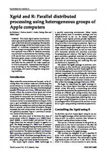
Figure 2a is the responsesurfacefor the two-variableBP-PDP model, and Figure2b is the responsesurfacefor the corresponding logisticregression.The two graphsrevealedseveralinterestingfeatures.First, for certaincombinations of dbhanddbhincrement,the BP-PDP modelactuallyfollowedsomeformsof a logisticcurve. This is rather interestingsince, unlike logisticregression,the systemwasnot instructedto fit a logisticcurvebut to onlyminimizethe squared errors.This findingimpliesthata mortalitycurve(or survivalcurve)mayindeed be best describedby the logisticfunction,basedon the goodness-of-fit measure (i.e., SSE) employed.One mightarguethat even thoughthe systemwas not instructedto fit logisticcurvesto the dataexplicitly,throughthe use of a logistic transferfunctionthe systemwasinstructedto fit logisticcurvesimplicitly.Using a logistictransferfunctionin a BP-PDP systemis merelya convention becauseit hasdesirableproperties(e.g., avoiding noisesaturation,easyto calculateweight changes,etc.), just asin manystatisticalanalysesthe errorsare requiredto follow a nonual distribution. Such transfer function h•asbeen used in other areas where

the nature of the problemsh•aveno bearingon the logisticfunction,suchas characterrecognitionproblems.Other functionscan alsobe used as transfer functions(Williams1986). The secondinterestingfeaturerevealedby the two responsesurfacesis related to the abilityof generalization of eachmodel,i.e., a model'sabilityto handlenovel cases.First, for combinations of largedbhandlargedbhincrement,the response surfacefrom the logisticregressionshoweda downwardtrend, meaningthat the

AUGUST 1991/877

probability of survivalover a 5-yearperiodfor a largetree with largedbhincrement tends to be lower than that of trees with the same size but with smaller dbh

increments.In contrast, the responsesurfacefrom the two-variableBP-PDP modelremainedilar at thatregion,with estimatedprobabilities of survivalaround 0.98. This downwardtrendin the responsesurfacefromthe logisticregressionis dueto the significant negativeparameterestimatefor the interactionterm in the model.

Figure3 showsthe relativesurvivalrate in dbhanddbhincrementcombinations in the actual data. First, it can be seen that the responsesurface from the two-variableBP-PDP systemactuallyfollowedthe observedrelativesurvivalrate

878/FOgl•rSC•CE

1.0

0.4

0.2

0

1.0

0.8

0.6

0.4

0.2

0.0

DBH INCREMENT

(NORivlALIZED) FIGU• 3.

Relative surdval rate in the actualdata. Data are groupedinto a 0.2 interval on the

normalized scales for both dbh and dbh increment.

muchmore closelythandid that of the three-parameterlogisticregression.Only a few dead trees in the data set are in the regionof large dbh and large dbh increment.These few deadtrees causedthe logisticmodelto have a significant negativeinteractiontenn. The BP-PDP systemperformsbetter in estimatingthe survivalprobabilities of thesenovelcases.No matter what the dbhsize classis, if everythingelseis equal,a tree with a largedbhincrementshouldhaveat least the same,likelya higher,probabilityof survivalthantrees with the samedbhbut smallerdbhincrements.Second,for combinations of the wholerangeof dbhand smalldbhincrements,the two modelsalsoresponded quitedifferently.If we set the normalizeddbhincrementto be 0.0 (0.1 in. over a 5-yearperiodin the original scale),thenthe estimatedsurvivalprobabilities over a 5-yearperiodfor the whole range of dbh from the BP-PDP modelare around0.5. In comparison,the estimatedprobabilities of survivalfromthe logisticregression rangedfromalmost0.0 to 1.0. Sincethe majorityof the combinations mentionedabovedonot exist in the actualdata,the questionis whichmodelis morereliable.In the caseof smalldbh, we donot havea definiteanswer,dueto the factthat the knowledgein smalltree dynamics is very limited.It shouldbe pointedout that, in general,smalltrees are rather robust and can surviveunderunfavorableconditionsas long as there is enoughincrementalgrowth. In this respect, the predictionsfrom the logistic model are rather conservative.Determiningwhichmodelis more accuratein predicting the survivalprobabilities of smalltreesreliesonfurthermonitoring. As for large dbh and smalldbh increments,the logisticregressionpredictedhigh survivalprobabilities whereasthe BP-PDPmodelgavesuchcombinations onlyan even chanceof survival.Again,it is difficultto determinewhichmodelis more accurate.

Using an approachsuch as PDP offers some advantagesover the logistic regression.For instance,it is well knownthat in modelingindividualtree mor-

AUGUST1991/ 879

tality, tree size andincrementalgrowthare not the only factorsthat determine tree survival.Other factorssuchas tree vigoror conditioncanalsohavegreat influenceon tree survival.However, sincesuchmeasurementsare usuallysubjective and/orqualitative,problemsarisewhenincludingsuchfactorsin a statisticalmodel.On the otherhand,as longas we canthinkof appropriate representationschemesfor suchfactors,we canput theminto usein a PDP system.The three-variableBP-PDP modelis a casein point.Whenthe variablepercentsoundnesswasintroduced intothe model,the BP-PDPapproach hada largerdropin the totalsumof squarederrorsthandidthelogisticregression. Sucha decreasein the sumof squarederrorsis especially noteworthy(about5%) in the deadtree group. In this case,the BP-PDP modelmadebetter useof the new informationthandid the logisticregression. Anotheradvantageof the PDP approachis in its flexibilityin fittingthe data.In someregionsof the data, even thougha nonlinearfunctionmay not be the best functionto describethe regions,a nonlinearregressionhasno other alternative butto fit the functionthroughthosedatapoints.On the otherhand,a PDP model may fit differentparts of the data with functionsof differentformssincesucha systemis not constrained by the structuralform of the minimizingfunction.This flexibilitymaybe valuablein modeling individual tree mortality. Currently,major impedimentsto the wide adoptionof the PDP approachfor solvingnonlinearproblemsinclude:(1) on conventional serialmachinesthe speed of convergence duringtrainingcanbevery slow,and(2) thereis noguaranteethat the systemwill settle in the optimalstate. The first is not so criticalsincethe advancements madein computertechnology havemadeparallelmachinesbecome moreandmoreavailableto the generalpublic.If a PDP systemis nm ona parallel machine,then the computation time requiredcanbe drasticallydecreased.What is importantis howto preventa PDP systemthatutilizeshack-propagation learn-

ing-algorithm, or any learningalgorithmfor that matter, from settlinginto a nonoptimal set of solutions.One approach is to designappropriate learningproceduresby eitheradjustinglearningrate throughtime or introducing smallperturbations intothe systemduringthe training.The problemwithsuchpracticesis thatno guidance existson settingupthe trainingschedule,andas yet thereis no guaranteethat the system will not settle into a nonoptimalstate. Recently, Wasserman(1989) has suggestedthat combining back-propagation and random optimization (statistical) learningmethods(suchas Boltzmann trainingprocedure, HintonandSejnowski1986)canreducethe trainingtime as well as ensuringthe systemto convergeto the optimalpointof the error function.It canbe expected thatin the nearfuturemorelearningalgorithms of thissort willbecomeavailable. There are alsoother hurdlesthat need to be overcomein applyingthe PDP approach to modelmortalityandothermodelingtasksin forestry.0nly a few of them will be discussedhere. As mentionedearlier, currentlynmninga PDP systemon serialmachines is time consuming. This willin turnmakeconventional model-testing procedures suchas cross-validation impossible to carryout. Thus, the needto developsomenew empirical andfeasiblemodel-testing procedures is clear. Second,more often that not the data used for modelingindividualtree mortalityare fromunequaltime intervalinventories.Then, it mustbe detenuined how this featureis incorporated into a PDP system.Third, otherlearningproceduresbesidesthe back-propagation methodshouldbe consideredas well. In certain respects, if the mortality problem is treated as a pattern completion

problem,thenit is possibleto usesomeformof unsupervised learningto accomplishthe desiredtask. Suchan approachmay broadenthe searchof possible methodsfor modelingindividualtree mortality.Finally,unlikeany other wellestablished methodsfor modeling,it is difficultto understand whatkindof knowledge a PDP systemactuallyextractedfrom the input data set, i.e., what do differentactivationpatternsrepresentin a trained systemand what are the meaningsof thoseweights?Can a trainedPDP systemtell us somethingnew aboutthe underlying mechanism of mortality?Suchdifficultyprobablyis the most crucialproblemthat needsto be workedon, sincefailureto answerthe questions will hinderthe adoptionof a PDP systemas a new modelingtechnique.

This studyis a first step in the directionof usinga PDP systemto modelregular noncatastrophic individualtree mortality.The studydemonstratedthat suchan approachis promisingin comparison to the widelyusedlogisticregressionapproach.Besidesbetter performance,it alsohas someadvantagesover the traditionalstatisticalmethods.However,manytopicsremainto be addressedbefore we can confidentlyand fully utilize the advantagesof the PDP approachas an alternativemethodfor modelingindividual tree mortality.

BELCHER, D., M. HOLDAWAY, and G. BP, AND.1982. A description of STEMS: The standandtree evaluation andmodeling system.USDA For. Serv. Gem Tech. Rep. NC-79. 18 p.

GERT•ER, G. 1989. The needto improvemodelsfor individual tree mortality.P. 59-61 in Proc. SeventhCentralHardwoodConf. USDA For. Serv., Carbondale,IL.

GOP, MA•, R.P., andTJ. S•sowsrd. 1988. Analysisof hiddenunitsin a layerednetworktrainedto classifysonartargets.NeuralNetwork 1:75-89.

HAMILTOS, D.A., JR.,andB.M. EDWARDS. 1976.Modeling theprobability ofindividual tree mortality. USDA For. Serv. Res. Pap. INT-185.22 p.

HINTON,G.E. 1989. Connectionist learningprocedures. Artif. Intel. 40:185-234. HINTOS,G.E., andT.J. SF.•OWSrd. 1986.Learningandrelearning inBoltzmann machines. P. 282-317 in Paralleldistributedprocessing: Explorations in the microstructure of cognition.Vol. I. Rumelhart, D.E., andJ.L. McCleHand (eds.). MIT Press,Cambridge,MA. HORNIK, K., M. STINCHCOMBE, andH. WHITE.1989. Multilayerfeedforward networksare universal approximators. NeuralNetwork 2:359-366. L•EDES,A., andR. FA•ER. 1987.Nonlinearsignalprocessing usingneuralnetworks:Prediction and systemmodelling. Los AlamosNat. Lab. Tech. Rep. LA-UR-87-2662.34p. LECUN,Y. A theoretical frameworkforback-propagation. 1989.P. 21-28 in Proc.1988Connectionist ModelsSummerSchool,Touretzky,D., G. Hinton,andT. Sejnowski (eds.).Morgan-Kauffnan, San Mateo, CA.

RUMELH•T,D.E., andJ.L. McCLELLASD (eds.). 1986.Paralleldistributed processing: Explorations in the microstructureof cognition.Vol. I. MIT Press, Cambridge,MA.

RUMELHART, D.E., G.E. HINTON, andRJ. WII.LI•4S. 1986.Learning internalrepresentations by error propagation. P. 318-362 in Paralleldistributed processing: Explorations in the microstructure of cognition. Vol. I. Rumelhart,D.E., andJ.L. McCleHand (eds.). MIT Press,Cambridge,MA. SASINSTITUTE INC. 1983. SUGI Supplemental LibraryUser'sGuide.SASInst., Inc., Cary, NC. SOMERS, G.L., ETAL. 1980.Predictingmortalitywith a Weibulldistribution. For. Sd. 27:291-300.

AUGUST 1991/ 881

WASSERMAN, P.D. 1989. Neuralcomputing: Theoryandpractice.Van NostrandReinhold,New York.

WHITE,H. 1989a.Neural-network learningandstatistics.AI Expert4(12):48-S2. WHITE,H. 1989b.Someasymptotic resultsfor learningin singlehidden-layer feedforwardnetwork models.J. Am. Star. Assoc.84:1003-1013. WILLIAMS, R.J. 1986. The logicof activation functions. P. 423-443 in Paralleldistributed processing: Explorations in the microstructure of cognition.Vol. I. Rumelhart,D.E., andJ.L. McCleiland (eds.). MIT Press, Cambridge,MA. Copyright1991by the Sodetyof AmericanForesters ManuscriptreceivedFebruary2, 1990

The authorsare Ph.D. studentand AssociateProfessorof Forest Biometrics,Dept. of Forestry, Universityof Illinois,1301W. GregoryDrive, 110 MumfordHall, Urbana,IL 61801.This studywas partiallysupportedby Mclnlire-StennisProjectMS FOR 55-320 andby the U.S. Army Construction EngineeringResearchLaboratory.

In this appendix,the necessaryequationsfor the back-propagation algorithmare formallyderived.Thisalgorithmreceivedits namefromthe wayit handleserrors generatedby the system,i.e., it will propagatethem backwardfrom the output layer throughhiddenlayer(s)to the inputlayer of the system.It shouldbe noted that thoughthe derivationsof the BP algorithmhave been reportedin other publications, in thisappendixa differentapproach is employed,andit shouldhelp the readersunderstandthe essencesof BP algorithm.This appendixis divided into two parts. In the first part it will be shownhow errors in a back-propagation modelare back-propagated. In the secondpart, equationsfor changinga weight according to the localerror derivedin the first part will be presented.However, technicaldetailswhichneed to be consideredin actualimplementationof the algorithmwill not be discussed in this appendix.Interestedreaderscan consult Rumelhart, Hinton, and Williams(1986) for more information. DERIVATION OF Loc•

EI•ORS

Let

Xj(L)betheoutput valueofthejth processing inthe Lth layerof a back-propagation PDP system

Wii(L)betheweight connecting theithunitinthe (L - 1)th layer andthe jth unit in the Lth layer

Ii(L) betheweighted sumofinputs to thejth unitsin layerL, i.e.,

Ii(L) = •Z[W•i(L) . X,(L- 1)] Also assuming 1. 2.

there is a globalerror functionE, there is a differentiableactivationfunctionf,' and

882/Fo•.sTSQF•CE

(1)

3. the outputof a unitis equalto its activationvalue,then

X•(L) -- .•I•(L)] Equation(1) is for propagating inputinformation forwardthroughthe system, andwe want to establisha relationshipbetweena particularunit andunitsin the layer aboveit for back-propagation of errors in the samemanneras (1) is for forwardinputthroughthe system.First, define

8i(L)= - aE/ali(L)

(2)

asa measureof localerror for unitj in layerL. The reasonfor thisto be a measure of local error will be shownbelow. Intuitively, sinceany output from a PDP systemis a functionof connection weightsandactivationvalues,then any error a systemgeneratesmustalsobe a functionof thesetwo variables.We now want to express(2) in terms of weightsbetweenthis particularunit andthe unitsin layerL + 1, andalsoin terms of localerrors for unitsin the layer aboveit. By usingthe chainrule, we have

-BE

O•Ij(L)]

8,(L) =O•I,(L)] ' -•E

= aX,(L•'œ[I,(L)]

(3)

Usingthe chainrule again,the first componentof (3) canbe written as

='-aE/•{a•[W•,(L+i)'Xi(L) J

-- • [a•(L + 1}.•(L + 1)1

(4)

By substituting(4) into (3), we now have

a•(L) = • [8•(L + 1). •(L + 1)]./'[Ij(L)]

(5)

whichis in the desiredform. Therefore, we have establisheda methodfor backpropagating errorsfrom onelayer to the layerimmediatelybelowit. It shouldbe notedthat (5) is for nonoutput layersonly,sincewe needthe existenceof layer L + 1 for thisequation to workproperly.By examining (5) and(1), we seethatthe summation term in bothequationsis rather shnilar,exceptthat in (1), we havea weightedsumof inputsignalsfromunitsin thelayerimmediately below,andin (5)

AUGUST 1991/ 883

we have a weightedsum of local errors from the layer immediatelyabove a particularprocessingunit. If we consider(1) as the contributionof a processing unit to the system,then (5) is the responsib/lity of a unit to the system. Now we needto showhowerrorscanbe back-propagated fromthe outputlayer to the hyer belowit. First, let us assumethat there is a globalerror functionin the systemfor a particularinputpatternp, anddefineit as

zp: m.

-

2

(6)

y

whereT•.istheoutput ofcomponent j inthetargetoutput vector,andO½isthe outputof component j in the actualoutputvector.This error measureis similar to the leastsquarecriterionin virtue.Thenby (2), the localerror for unitj in the outputlayer is

8i(0) = - aEt,/ali(O) = (-oEfO•).[oOm./oly(O)] = -

(7) (8)

whichis onlythe differencebetweenthe targetandthe actualvaluesmultipliedby a factor.Andfromthisequation,we cansee that (2) is indeeda measureof local error. Equation(8) is for the globalerrorof a particularpattern.We candefinean overallglobalerror as

p

whichmeansthat the globalerror will be minimizedif eachand every pattern's error is minimized.

Duringthe derivationof localerror, we assumedthat there existsa differentiable activationfunctionf. Amongmany suchfunctions,one that is most frequentlyemployedin a back-propagation PDP systemis the logisticfunction(or sigmoidfunction).If in a systemthe activationfunctionis indeeda logisticfunction, i.e., f(x) = 1/(1 + e-•) then

f(x) = f(x) ß[• - ?ix)] and (5) can be written as

gj(t)= Z [g•(L + 1)' I•(L + 1)].{Xj(L) ß[1- Xj(L)] } k

andgi(L)israthereasyto calculate underthiscondition. ADJUSTING CONNECTION WEIGHTSACCORDING TO Loc•

ERRORS

In this section,we will show how the back-propagation algorithmuses the so-

calledgeneralizeddelta rule to minimizethe globalerror by adjustingweights accordingto localerrors.

884• Fov•rsc•cE

LetAWjibetheweightchange of Wji.Thedeltaruleis defined as = I•' a• ßIt•

(9)

where

I• is a constantof proportionalityrepresentingthe learningrate,

T• isthetargetoutput forpattern p, O• is theactual output forpattern p, and Ipiis theinputvalueof theith component ofpattern p. Basically, thisrulestatesthata weightwillbeincreased or decreased according to the differencebetweenthe targetoutputandthe actualoutputvalue.It canbe shownthat if the error functionfor patternp is definedas (6) then

-OEp/ OWji= apj. Ipi whichis proportional to AWji as prescribedby the deltarule. However,this delta rule is onlyapplicable to a linearsystem,i.e., for a systemwith a linearactivation function.This type of systemcanonlybe usedto solvea certainclassof problems.Thus, for systemswith hiddenunitsandnonlineartransferfunction,suchas a back-propagation system,we need to generalizethe abovedeltarule. Let

a%i(œ)= -

ß

(10)

where [3 is a learningcoefficientwhichis usuallya positivenumbersmaller than 1.

Equation(10) canbe expressedin terms of localerror as follows:

OEp/OWji(L ) = [OEp/OIj(L)]. [O[(L)/OWji(L)] = - •(L) ßXi(L- 1) and thus

aW•,(œ)= • ßaj(œ).X,(œ- 1)

= [3.• [g•(L + 1). I4•(L+ 1)].f'[Ij(L)].X,(L- 1)

(11)

Equation(11) is the generalformof the generalized deltarulefor a systemwith hidden units and a nonlinear activation function.

To summarize,the back-propagation algorithmis a recursivemethod:the system is first presentedwith aninputvector,andthe vectoris propagated forward throughthe systemto the outputlayerusing(1); thenthe error is calculated and back-propagated fromthe outputlayerto theinputlayerusing(5), andnecessary weightadjustments are madeusing(11).

AUGUST1991/ 885