A Simulation-based XML Routing Synopsis in Unstructured P2P Networks Qiang Wang Univ. of Waterloo, Canada
[email protected]
Abhay Kumar Jha∗ IIT, Bombay
[email protected]
¨ M. Tamer Ozsu Univ. of Waterloo, Canada
[email protected]
Abstract Many emerging applications that use XML are distributed, usually over large peer-to-peer (P2P) networks on the Internet. The deployment of an XML query shipping system over P2P networks requires a specialized synopsis to capture XML data in routing tables. In this paper, we propose a novel graph-structured routing synopsis, called kd-synopsis, for deployment over unstructured super-peer based P2P networks. This synopsis is based on length-constrained FBsimulation relationship, which allows the balancing of the precision and size of the synopsis according to different space constraints on peers with heterogeneous capacity. We report comprehensive experiments to demonstrate the effectiveness of the kd-synopsis.
1
Introduction
In recent years, Peer-to-Peer (P2P) architecture has become a popular decentralized platform for many Internetscale applications such as file-sharing1 , instant messaging2 , and computing resource sharing3 . Meanwhile, XML data are increasingly used as a format for data exchange and storage on the Internet, such as XML-based sensor data [17] and Web service data defined in WSDL and SOAP. Thus, it is increasingly important to process queries efficiently over data deployed in large-scale P2P networks, where centralized catalogs are not always available and peers may join and leave arbitrarily. Distributed (XML) query processing can follow either data-shipping or query-shipping approaches. While data shipping moves data to a query processing site, query shipping systems route queries to where the data are located for processing. Query shipping is preferable in P2P systems because it can exploit the computational power of peers to process queries in parallel, and the cost of sending queries is usually much smaller than that of sending data. Query shipping strategies vary based on different P2P overlay network architectures and routing protocols. In structured P2P architectures, data are placed on peers that are organized in a structured overlay network by using distributed hashing, and each peer manages, along with data, hash-based routing information for “neighboring” peers. In contrast, unstructured P2P architectures keep data on original peers and route queries either by flooding (e.g., Gnutella v0.4 [3]) or by using super-peers (e.g., Gnutella v0.6 [4]). While flooding is effective when searching popular data with a lot of replicas [26], a super-peer based architecture makes routing more efficient by organizing peers hierarchically where upper-level peers maintain information about the content of their lower-level ones and use this for routing. Such an architecture combines the advantages from both centralized systems (e.g., the exploitation of heterogeneity of peers) and distributed systems (e.g., scalability and robustness), and has been employed in real P2P file-sharing systems [6, 7]. ∗ Work
done while the author was visiting the University of Waterloo. http://www.gnutella.com 2 Skype: http://www.skype.com 3 Seti@home: http://setiathome.ssl.berkeley.edu 1 Gnutella:
1
In this paper, we focus on XML query routing in query-shipping P2P systems under super-peer based overlay network architectures. More specifically, we propose an effective XML synopsis that can be used for maintaining routing state. For the sake of simplicity, we assume that each peer contains a tree-structured XML document (i.e., without ID or IDREF). In the case that a peer has multiple documents, we can model them under a virtual root. We are concerned with a commonly used subset of XPath [14], called Branching Path Query (BPQ) [22]. Briefly, BPQ covers self, child, descendant, descendant-or-self, parent, ancestor and ancestor-or-self axes. Moreover, we consider the conjunction (i.e., and operator) of predicates. Since we do not consider negation in queries, we actually work on a subclass of BPQ, defined as BPQ+ [31]. Our solution, called kd-synopsis, is a graph-structured synopsis over XML data that can easily balance its precision and size. The k and d are length constraints to be imposed over the Backward and Forward-simulation relationships (Section 2), which are theoretical foundations of our routing synopsis. To be more specific, our major design novelties are as follows: • Most proposed routing state data structures are simple, such as the pair of used in file-sharing P2P systems, or the used in Internet routing. These simple routing states usually capture, quite precisely, the information necessary for routing, and small-sized routing tables improve the scalability of the system with respect to both the storage size and the routing decision making process. However, XML data are much more complex, requiring a hierarchically-richer synopsis to capture its information. Furthermore, modern P2P systems are heterogeneous, in that different peers have different capacities including storage space size4 , which requires a more adaptive routing state representation whose size can be easily adjusted. Kd-synopsis better captures XML hierarchical information, while using a length-constrained FBsimulation relationship to control the size of the synopsis. • The organization of the routing synopsis into routing tables is nontrivial, because it is not straightforward to aggregate synopses from multiple peers. In particular, for kd-synopsis, this is more critical since each peer’s routing synopsis may have different k and d values. In this work, we propose a method to aggregate multiple kd-synopses into a routing state organized as a sequence of synopses ordered by k and d values, which keeps the precision of the synopses as much as possible with respect to specific space constraints. Consequently, the contributions of this paper consist of three parts: First, we give the first formal definition of length-constrained FBsimulation relationship over XML data, which we call kd-simulation. Second, we develop a novel size-adjustable routing synopsis, named as kd-synopsis. Finally, we address the aggregation and update maintenance issues for routing tables consisting of kd-synopses, and demonstrate the effectiveness of our design with extensive experiments. The organization of the paper is as follows. We introduce the background and related work in Section 2. In Section 3 we precisely define the kd-simulation relationship and address the generation of kd-synopses over XML documents. Section 4 focuses on the XML query shipping enforced in super-peer based unstructured P2P networks. Experimental results are presented in Section 5, demonstrating the effectiveness of our routing synopsis. Finally, we conclude in Section 6.
2
Related Work and Background
2.1 Related Work XML query shipping problem is addressed in both structured [19, 16, 18] and unstructured P2P [24] domains. Since we are interested in unstructured P2P systems in this paper, Koloniari and Pitoura’s work [24] is the most relevant, where Bloom filters are used to capture the set of elements on document tree levels and paths with same lengths. The basic idea is to encode the set of all the elements on each document level into a specific Bloom filter (the Breadth Bloom filter), and encode the set of all the linear path strings with a fixed length into a specific Bloom filter (the Depth Bloom filter). For example, Figure 1 shows the Breadth and Depth Bloom filters of an XML document that adheres to the DTD in the figure. Here the Bloom filters are presented in rectangles while their corresponding set of elements or paths are attached next to each entry for clarity. For simplicity, we use the first characters to represent element names. 4 This
space especially indicates main memory space used to store routing information.
2
Figure 1. A Bloom-filter based synopsis Although Bloom filter is space efficient in checking membership over a set of elements, it has several disadvantages when used to encode hierarchically-rich XML data. First, it cannot precisely encode the ancestor-descendant relationship among elements, because Breadth Bloom filter does not capture the parent-child relationship among nodes at different levels, and Depth Bloom filter only captures linear XML paths with specific lengths by uniform hashing. Thus a query with ancestor-descendant axis cannot be checked against the data effectively. For example, using the Bloom filter synopsis proposed in [24], the query “c//n” will be falsely determined as positive against the document in Figure 1 (a query is positive to a document if the evaluation result is non-empty). Second, to guarantee that there are no false negatives, which is desirable in query shipping systems, each document level has to correspond to a Breadth Bloom filter, so the size of the synopsis increases sharply when used to encode deep-structured documents, such as those following a recursive schema [25]. Finally, each peer in the system needs to use the same hash functions and agree on the size of the Bloom filters (i.e., size of bit sequences of the Bloom filter) corresponding to a specific level or a fixed path length. This may not be feasible in large heterogeneous P2P systems. In this work, we develop a graph-structured synopsis to represent routing state, which can capture the XML hierarchial information more easily and is size-adjustable so as to fit the heterogeneous capacity on different peers. Compact graph-structured synopses have been developed to index XML data. Milo et al. employ Forwardbisimulation equivalence relationship (described in Section 2.2) to devise a reduced index for XML data [27] with respect to linear path XML queries. Polyzotis et al. develop XSketch synopsis for selectivity estimation, which also exploits the Bisimulation relationship to reduce the common structures in XML data [30]. Further, Ramanan proves that FBsimulation quotient is the smallest covering index5 of XML data with respect to BPQ+ queries [31], and the quotient can be much smaller than Bisimulation-based synopses. Kd-synopsis shares the graph structure of these synopses and builds on the same foundation of the FBsimulation relationship, but it can be significantly smaller than FBsimulation quotient. Moreover, to make the routing synopsis size-adjustable according to the heterogeneous capacity on different peers, we impose length constraints over the FBsimulation relationship such that we can easily balance the size and the precision through the constraint parameters. Kaushik et al. also consider a length constrained equivalence relationship (i.e., k-bisimilarity) in their A(k)index for XML indexing [23], but they impose length constraints only on the backward direction of the Bisimulation relationship, such that document nodes with different subtree structures can not be distinguished, leading to a less precise synopsis for BPQ+ queries. Homomorphic Compression has been proposed to encode XML data into a compressed form. Tolani et al. propose the XGrind system, which employs dictionary encoding and Huffman encoding to compress tags and data values respectively [32]. Min et al. use reverse arithmetic encoding to compress XML linear paths in the XPress system [28]. While both of the compression schemes provide reduced queriable XML data encodings, they do not compress structures of original XML data, so basically they are orthogonal work and their encoding strategies over element names can be applied directly over our kd-synopsis. 5 An index DI of document D is a covering index with respect to a query set if no query in the set can distinguish between two nodes of D that correspond to the same indexing node in DI.
3
2.2 Background FBsimulation relationship has been shown to capture similar structures in XML data for BPQ+ queries [31]. We use it as the theoretical foundation of kd-synopsis to remove redundancy with respect to the positive check6 of BPQ+ queries. FBsimulation is an extensively researched concept, which is used to describe the structure of semi-structured data [13], and has recently been employed to build compact covering indexes for XML data [31]. Given a directed graph G = (V, E), where V is the node set and E is the edge set, for a node v ∈ V , let label(v) return the label of v. Then • Backward-simulation (¿B ) is a binary relation over V 2 , such that, ∀u, v ∈ V , u ¿B v iff – label(u) = label(v); – for every parent node u0 of u in G, there is a parent v 0 of v such that u0 ¿B v 0 . • Forward-simulation (¿F ) is a binary relation over V 2 , such that, ∀u, v ∈ V ,u ¿F v iff – label(u) = label(v); – for every child node u0 of u, there is a child v 0 of v such that u0 ¿F v 0 . • FBsimulation is a binary relation (¿F B ) over V 2 , such that ∀ u, v ∈ V , u ¿F B v (called u is FBsimulated to v) iff – label(u) = label(v); – for every child node u0 of u, there is a child v 0 of v such that u0 ¿F B v 0 ; – for every parent node u0 of u, there is a parent v 0 of v such that u0 ¿F B v 0 . Specifically, with respect to an XML document tree, if node u is FBsimulated to node v, two properties will hold: first, the incoming path starting from the document root to u exactly matches that from the document root to v; second, for any node u0 on the matching incoming path (including u itself), all subtree patterns rooted at u0 can be found in the subtrees rooted at v 0 , which is u’s counterpart node on the matching incoming path affiliated with v. For example, consider a document tree shown in the Figure 2, where we use subscripts to distinguish nodes with same labels for demonstration (i.e., c1 , c2 , c3 all have label c). While t2 is FBsimulated to t4 , t1 is not FBsimulated to t4 because they do not share matching incoming paths. Similarly, s1 is FBsimulated to both s2 and s3 , while s2 is not FBsimulated to s4 because they have distinct subtree patterns. Once a node is FBsimulated to the other, the former becomes redundant when used in the positive check of BPQ+ queries against documents. For example, given a query /b/c/s, we can correctly determine that the query is positive to the document in Figure 2 without considering s1 . We will exploit this finding to build the kd-synopsis later.
Figure 2. An XML document tree FBsimulation quotient is a FBsimulation-based synopsis that can be used as a covering index of XML data with respect to BPQ+ queries. Briefly, nodes FBsimulated to one another are merged so as to build a smaller sized index to answer BPQ+ queries. For example, in the XML document shown in Figure 3, s2 and s3 are merged into the same node in the FBsimulation quotient because they are FBsimulated to each other, while s1 is not collapsed because it is not FBsimulated to any node. While distinguishing s1 from other nodes is crucial for answering queries precisely, it is unnecessary when we are concerned with the positive check of queries, where we only care whether a query can be answered by the data. Thus we can take a more aggressive reduction strategy than FBsimulation 6 The
check of whether the result set of evaluating a query against a document (or a synopsis) is non-empty.
4
quotient, which will be addressed in Section 3. Moreover, in a heterogeneous P2P environment, peers have different capacities to store routing information, such that we need a strategy to adjust the size of the synopsis dynamically, which requires an elegant way to trade off the precision of the synopsis.
Figure 3. FBSimulation quotient
3
kd-synopsis
An XML routing synopsis should satisfy two properties to be effective in P2P environments. First, it should be as precise as possible such that the routing synopsis can discriminate queries accurately – this will save the communication cost since false positive queries7 will not be routed. Second, the routing synopsis should adapt to heterogeneous capacities (i.e., storage space for routing information) on different peers. In this Section, we describe kd-synopsis, a novel routing synopsis that is based on kd-simulation, a length-constrained version of FBsimulation relationship. Through the adjustment of length constraints over kd-simulation, kd-synopsis can acquire a level of precision with respect to specific size constraints.
3.1 Definition of kd-simulation In this section, we define kd-simulation relationship that can identify XML element nodes that have similar structures within the specified incoming and outgoing levels. Specifically, based on the notions of Backwardsimulation, Forward-simulation, and FBsimulation, we define their length-constrained variants: k-Backwardsimulation, d-Forward-simulation and kd-simulation. • Given a graph G = (V, E), k-Backward-simulation (¿kB ) is a binary relation over V 2 defined inductively as follows (k ≥ 0). Given u, v ∈ V ,, – u ¿0B v iff label(u) = label(v); – u ¿kB v iff (1) label(u) = label(v); (2) for every parent node u0 of u, there is a parent v 0 of v such that u0 ¿k−1 v0 . B • Given a graph G = (V, E), d-Forward-simulation (¿dF ) is a binary relation over V 2 defined inductively as follows (d ≥ 0). Given u, v ∈ V , – u ¿0F v iff label(u) = label(v); – u ¿dF v iff (1) label(u) = label(v); (2) for every child node u0 of u, there is a child v 0 of v such that u0 ¿d−1 v0 . F Briefly, k-Backward-simulation identifies similar incoming paths within k XML tree levels, while d-Forwardsimulation identifies similar outgoing structures within d XML tree levels. For example, in the XML document tree shown in Figure 2, t1 ¿0B t2 holds because they share the same label, but t1 ¿1B t2 does not because they have different parents (i.e., different incoming edge one level away); c2 ¿1F c3 holds but c2 ¿2F c3 does not hold because they have distinct outgoing edges two levels away (i.e., s/t and s/p respectively). Now we define kd-simulation as a reflexive and transitive relation over V 2 , with k and d values as the length constraints over Backward and Forward-simulation relationship respectively. 7 A query is false positive when it is determined as positive to the synopsis while it is actually negative to the data on which the synopsis is generated.
5
• Given a graph G = (V, E), kd-simulation (u ¿(k)(d) v, called u is kd-simulated to v) is a binary relation over V 2 defined inductively as follows. Given u, v ∈ V , – u ¿(0)(d) v iff label(u) = label(v) and u ¿dF v; – u ¿(k)(0) v iff label(u) = label(v) and u ¿kB v; – u ¿(k)(d) v iff (1) label(u) = label(v); (2) for every child node u0 of u, there is a child v 0 of v such that u0 ¿(k)(d−1) v 0 ; (3) for every parent node u0 of u, there is a parent v 0 of v such that u0 ¿(k−1)(d) v 0 . For example, in the Figure 2, t4 is kd-simulated to t6 with respect to k = 1, d = 1 because their parent nodes c2 ¿(0)(1) c3 , and neither of them has children nodes. However, t4 is not kd-simulated to t6 anymore under k = 1 and d = 2, since c2 ¿(0)(2) c3 (i.e., c2 ¿2F c3 ) does not hold. Note that when both k and d are equal to G’s graph diameter (i.e., the tree depth when G is an XML document tree), kd-simulation evolves into the FBsimulation relationship, which is the basis of the covering index graph for BPQ+ [31], and when both k and d are equal to zero, it degrades into the label-equivalence relationship, which is the basis of the label-splitting graph8 that captures all the basic label and edge information in G. Efficient algorithms have been designed to compute the Forward-simulation relationship among graph nodes [15, 21]. We propose an algorithm (Algorithm 1) to cover our special circumstances. This algorithm is similar to that given by Henzinger et al. [21], but has two important differences. First, instead of only Forward-simulation, we consider both Backward and Forward-simulation. Second, we apply length constraints over the FBsimulation relationship. The implementation is straightforward, containing iterations for the computation of d-Forwardsimulation (k-Backward-simulation), where in each iteration, the distinction among nodes incurred by different outgoing edges (incoming edges) are propagated to an upper (lower) level in the tree. It is more economical to put the computation of d-Forward-simulation before that of the k-Backward-simulation, because the latter computation can easily take into account the distinction of same-labelled nodes that do not have d-Forwardsimulation relationship. Otherwise, an extra step is needed to propagate such distinctions k levels down the tree. This asymmetry over the computation order is caused by the characteristic of the tree structure that each node has at most one incoming path while it probably has multiple outgoing edges. Since Algorithm 1 is a length constrained version of Henzinger et al. [21], the time complexity is still O(|V ||E|) with respect to the graph G. In the following, we give the correctness proof of the algorithm. Proof. Given an XML document tree D = (V, E) and u, v ∈ V with label(v) = label(u), if (v, u) belong to the kd-simulation relationship under k and d values, two sufficient conditions as follows: first, ∀pv that is the ancestor node of v that is within l (0 ≤ l ≤ k) tree levels from v, there exists a node pu as the ancestor node of u that is l tree levels away from u such that pv ¿(k−l)(d) pu ; second, ∀cv that is a descendant node of v that is within l0 (0 ≤ l0 ≤ d) tree levels from v, there exists a node cu as the ancestor node of u that is l0 levels away from u 0 such that cv ¿(k)(d−l ) cu . Consider the iteration (lines 12 to 15 in Algorithm 1), ∀x ∈ V , sim(x) (i.e, the set of the potential nodes that x is kd-simulated to) changes in each iteration according to its children nodes. We claim invariant 1 before the ith (1 ≤ i ≤ d) iteration: ∀y ∈ sim(x), x ¿(0)(i−1) y. Initially before the iteration, sim(x) contains all the nodes that share the same lable as x, so the invariant holds (i.e., ∀y ∈ sim(x), x ¿(0)(0) y). Then consider the ith iteration, let us assume that for a node y ∈ sim(x), there exist at least one child node cx of x such that there is no child node cy of y and cx ¿(0)(i−1) cy . Thus, in this ith iteration, y will be removed from sim(x) (line 18), such that after this iteration, it holds that ∀z ∈ sim(x), label(z) = label(x) and for any child node cx of x, there exists a child node cz of z such that cx ¿(0)(i−1) z, which leads to the conclusion that x ¿(0)(i) y, satisfying the invariant 1. As for the second iteration (lines 28 to 41), we claim another invariant (i.e., invariant 2) before each iteration: ∀y ∈ sim(x), x ¿(i−1)(d) y. Initially before the first iteration, the invariant holds because it is obvious that ∀y ∈ sim(x), x ¿(0)(d) y, resulting from the invariant 1. Then consider the ith iteration, and let us assume that before this iteration, ∀y ∈ sim(x), x ¿(i−1)(d) y, then in this ith iteration, for an node y ∈ sim(x), for a parent node of x, px , it there does not exist a parent node py of y such that ¿(i−1)(d) py , then y will be removed from the sim(x) (line 34), thus after the ith iteration, it holds that ∀z ∈ sim(x), label(z) = label(x) and for any parent node px of x, there exists a parent node pz of z such that px ¿(i−1)(d) pz . Meanwhile, after the ith iteration, it naturally becomes true that, for an arbitrary child node cx of x, there exists a child node cy of y such that cx ¿(i)(d−1) cy , because cx ¿(0)(d−1) cy holds according to invariant 1, meanwhile there is no distinction on 8 In
such a graph, nodes are merged if they have common labels, and edges are merged if they have common labels on both ends.
6
the incoming paths within i tree levels away (otherwise, y will be removed from sim(x) in this iteration by line 34). Consequently, if y still belongs to sim(x) after the ith iteration, x ¿(i)(d) y will hold, thus after k iterations, ∀y ∈ sim(x), x ¿(k)(d) y. Algorithm 1 compute kd simulation 1: 2: 3: 4: 5: 6: 7: 8: 9: 10: 11: 12: 13: 14: 15: 16: 17: 18: 19: 20: 21: 22: 23: 24: 25: 26: 27: 28: 29: 30: 31: 32: 33: 34: 35: 36: 37: 38: 39: 40: 41:
Input: G = (V, E), k, d Output: for each node v ∈ V , the set of vertices sim(v) such that sim(v) contains all the nodes v satisfying v ¿(k)(d) u Auxiliary functions: ∀x, y ∈ V , pre(y) = {x|(x, y) ∈ E}, post(x) = {y|(x, y) ∈ E} for v ∈ V do sim(v) ← the set of the vertices with the same label as v’s; end for ktmp ← k; dtmp ← d; //d-Forward-simulation for all v ∈ V do sim0 (v) ← sim(v); end for while dtmp > 0 do for all v ∈ V, u ∈ sim(v) do if ∃vc ∈ post(v), such that there does not exist uc ∈ sim(vc ), where uc ∈ post(u) then remove u from sim0 (v); end if dtmp ← dtmp − 1; for all v ∈ V do sim(v) ← sim0 (v); end for end for end while //k-Backward-simulation for all v ∈ V do sim0 (v) ← sim(v); end for while ktmp > 0 do for all v ∈ V, u ∈ sim(v) do if ∃vp ∈ pre(v), such that there does not exist up ∈ sim(vp ), where up ∈ pre(u) then remove u from sim0 (v); end if ktmp ← ktmp − 1; for all v ∈ V do sim(v) ← sim0 (v); end for end for end while
3.2 Building kd-synopsis In this section, we develop our new graph-structured synopsis (kd-synopsis) based on the kd-simulation relationship. Algorithm 1 already determines the kd-simulation relationship among document nodes, based on which we collapse an arbitrary graph node u to v (u 6= v) if u ¿(k)(d) v. This process continues until no node remains that can be kd-simulated by any other. Accordingly, an arbitrary edge e1 = (u1 , v1 ) is collapsed into e2 = (u2 , v2 ) if both u1 ¿(k)(d) v1 and u2 ¿(k)(d) v2 . Additionally, since absolute BPQ+ queries (i.e., queries starting from root level) require the synopsis to capture level information of the original document, we keep a mark for the kd-synopsis vertex9 that the root node of the original document is collapsed into. We propose Algorithm 2 to build the kd-synopsis for an XML document, where sim(v) is the set of all the nodes that v is kd-simulated to (i.e., the output from Algorithm 1). For clarity, we use V and E to denote the node and edge set of the original XML document tree, and use V and E to denote their counterparts in the synopsis graph. Briefly, we go through each node v of an XML document tree, and if there does not exist other nodes that v is kd-simulated to (lines 11 and 12), we insert it into f inal set; otherwise, we make sure that f inal set includes at least one node u that v is kd-simulated to (lines 15 to 19). Meanwhile, to facilitate the synopsis generation, we use ext(u) to track all the document tree nodes that are kd-simulated to u (line 20). After all the nodes are traversed, no nodes in f inal set will be kd-simulated to another one, thus we can build the kd-synopsis by generating a separate synopsis vertex for 9 To
distinguish from the nodes in original document trees, we use vertex when we refer to a node in kd-synopsis.
7
each node in f inal set and establish synopsis edges accordingly (lines 24 to 38). Figure 4 depicts the kd-synopses of the example document (Figure 2 and 3) under different k and d values. Note that in the kd-synopsis with k = 1 and d = 2, c3 is not collapsed because it has a distinct outgoing edge (i.e., s/p) two levels away. Algorithm 2 compute synopsis 1: 2: 3: 4: 5: 6: 7: 8: 9: 10: 11: 12: 13: 14: 15: 16: 17: 18: 19: 20: 21: 22: 23: 24: 25: 26: 27: 28: 29: 30: 31: 32: 33: 34: 35: 36: 37: 38:
Input: sim(v), a set of nodes that v (v ∈ V ) is kd-simulated to; G = (V, E), the original data graph Output: a kd-synopsis graph S = (V, E) Auxiliary function: ∀v ∈ V , label(v) returns v’s label. for all v ∈ V do sim(v) ← sim(v) − {v}; ext(v) ← {v}; end for f inal set ← φ; for all v ∈ V do if sim(v) = φ then f inal set ← f inal set ∪ {v}; else f inal set ← f inal set − {v}; if f inal set ∩ sim(v) = φ then choose any u ∈ sim(v); f inal set ← f inal set ∪ {u}; end if choose any u ∈ f inal set ∩ sim(v); ext(u) ← ext(u) ∪ ext(v); end if end for //generate synopsis vertices for all v ∈ f inal set do generate a synopsis vertex vs ; V ← V ∪ {vs }; establish a mapping from u ∈ ext(v) to vs ; if ∃u ∈ ext(v) that has no parent vertex in G then mark vs as a root; end if end for //establish synopsis edges for all e = (u, v) ∈ E do if ∃us , vs such that u maps to us and v maps to vs then generate a synopsis edge (us , vs ) in S; E ← E ∪ {(us , vs )}; end if end for
Figure 4. kd-synopsis The size of the kd-synopsis is bounded by the size of the original document, and the reduction ratio depends on k and d values. The smaller k and d are, the higher the reduction ratio will be, and in the extreme case when k = d = 0, the kd-synopsis is the same as the label-splitting graph. The time cost of Algorithm 2 primarily consists of three parts: first, The cost to building the f inal set, where the most expensive part is due to the set intersection between f inal set and sim(v) (line 15 and 19). In this work, we maintain the membership of each node u ∈ G in f inal set, such that the cost of the set intersection can be bounded by |V |, leading to a total cost of this part as O(|V |2 ). Second, since the extent set corresponding to the f inal set is a partition of V , line 27 is executed at most V times, so the generation of V (line 24 to 28) costs at most |V |. Third, the establishment of E (line 33 to 38) iterates over each edge in G, leading to a cost of |E|. In all, the time complexity of Algorithm 2 is bounded by |V 2 | + |V | + |E|, which is efficient. To demonstrate that our construction algorithm is optimum, we prove that the 8
kd-synopsis S constructed by Algorithm 2 has no redundant nodes that can be kd-simulated by others. To prove this, we argue that, given u, v ∈ G, first, when v ¿(k)(d) u while u ¿(k)(d) v does not hold, v will not be kept in S; second, when both v ¿(k)(d) u and u ¿(k)(d) v hold, at most one of them (actually the one to be first processed in Algorithm 2) will be kept in S. Proof. • According to the lines 11 to 21 of Algorithm 2, when vertex v is processed, if v ∈ f inal set and sim(v) is non-empty, then v will be removed, and a vertex u ∈ sim(v) (rather than v) will be kept in f inal set such that v ¿(k)(d) u; later even if u is replaced by another vertex w in f inal set, it always holds that ∃w ∈ f inal set such that v ¿(k)(d) w. Based on the property of the simulator set, ∀x ∈ V , if x ¿(k)(d) v, sim(x) contains all the vertices that v is also kd-simulated to, so ∀x processed after the removal of v, sim(x) ∩ f inal set 6= φ, thus v will never get a chance to enter f inal set any more. • Without loss of generality, let us assume that v is processed after u. When v is processed, if v ∈ f inal set, it will be removed according to Algorithm 2 (line 14); if u ∈ f inal set, then u will be kept in f inal set, rejecting v to enter f inal set later, as analyzed in proof of (1); or if u does not belong to f inal set when v is processed, there must be w ∈ V such that u, v ¿(k)(d) w, and since sim(v) 6= φ, w must belong to sim(v) ∩ f inal set, rejecting v to enter f inal set in the same way. kd-synopsis has two important properties: first, the synopsis has no false negatives when checked against BPQ+ queries; second, the synopsis maintains a well-defined precision that is determined by length constraints k and d. The first property is obvious, since when a graph node (i.e., document tree node) is collapsed into another, all its edge information is kept, which indicates that there is no loss of label or edge information in the synopsis. Note that we assume that root information is kept so that absolute BPQ+ queries can be checked correctly. With this guarantee, all data relevant to a query can be identified, which is desirable in query shipping systems. As for the precision of the synopsis, a kd-synopsis can be used to precisely check the positive of BPQ+ queries that can be characterized by kd-pattern, a parameter-constrained query pattern defined in the following. • (1)-descendant is a query pattern defined as child::c, where child is the axis defined in XPath, and c is an arbitrary label. (d)-descendant (d > 1) is a query pattern recursively defined as child::c[(d-1)-descendant]*. • (1)-ancestor is a query pattern defined as parent::p, where parent is an axis defined in XPath, and p is an arbitrary label. (k)-ancestor (k > 1) is a query pattern defined as parent::p[(k-1)-ancestor][(d)-descendant]*. • Then kd-pattern is a query pattern defined as x[(k)-ancestor][(d)-descendant]*, where x is an arbitrary label. Moreover, to model absolute BPQ+ queries, we can impose a root constraint over x. To visualize the kd-pattern, we illustrate it as a kd-pattern tree in Figure 5 (a), where pi denotes an ancestor element that is i edges away from x, and ci,j denotes the jth element on the i level of a (d)-descendant pattern tree. For future reference, the node labelled as x is called pivot of the kd-pattern tree. For example, given a BPQ+ query t[parent::c[child::s[child::t][child::p]]], its kd-pattern tree is shown in Figure 5 (b) where k = 1 and d = 2. Since the modelling of BPQ+ queries into kd-patterns is straightforward, we do not discuss it further in this paper. While the kd-pattern basically captures parent-child axis in BPQ+ queries, ancestor and descendant axes can also be modelled as kd-patterns if the document depth information is available. For example, given a query c[descendant::t] and the information that the depth of the documents to be queried over is up to three, the query can be modelled as three kd-patterns c[child::t], c[child::*[child::t]], and c[child::*[child::*[child::t]]] with k = 0 (i.e., no (k)-ancestor) and d = 1, 2, 3 respectively. Note here the “*” denotes wild card labels. Note, further, that kd-pattern tree is a general pattern tree not defined only for modelling queries, and we will use it to characterize a subtree in XML documents as well. The following theorem states that kd-synopsis maintains a well-defined precision with respect to the positive check of BPQ+ queries. Theorem 3.1. If a BPQ+ query can be modelled as kd-patterns (under k and d values), its positive/negative check against an XML document can be done correctly on all kd-synopses that are constrained by k 0 and d0 values, where k 0 ≥ max(k, d) and d0 ≥ max(k, d).
9
Figure 5. kd-pattern tree Proof. We first prove that all queries positive to documents will also be positive to their kd-synopses. Given a BPQ+ query q, let us consider a specific XML document D that q is positive to. q will definitely be positive to D’s arbitrary kd-synopses because we already claimed that kd-synopsis has no false negatives when checked against BPQ+ queries. Now we prove that if q is negative to D, while q can be modelled as a kd-pattern tree T under k and d values, it will also be negative to D’s kd-synopses under k 0 and d0 , where k 0 ≥ k and d0 ≥ d. If any node or edge in T does not exist in D, then q will be directly determined negative for all the kd-synopses because we do not add label or edge there. Thus let us assume that nodes labelled with x exist in D and focus on all the D’s kd-pattern (under k and d) subtrees that have a pivot node labelled as x (other kd-pattern subtrees will not affect the positive check of q). Consider nontrivial kd-patterns with k > 1 and d > 1 (the conclusion can be easily extended to kd-patterns with k ≤ 1 and d ≤ 1). Since q is negative to D, there exists at least one node in T that can not be satisfied by D, called the failure point (f p). There are two possible reasons for this failure. First, an edge incident to f p is missing from any D’s kd-pattern subtree that has the pivot node with the same label as x. Let us denote the missing edge as e = (ue , ve ) and consider an arbitrary D’s kd-pattern subtree S that includes another node ux with the same label as ue . Since S does not include e, ux will not have an edge that ends with another node that has the same label as ve , so ux is not kd-simulated to ue under k 0 > 1 and d0 > 1. Meanwhile, the unavailability of the pivot node within S, whose scope is bounded by k 0 and d0 , distinguishes ux from ue with respect to the kd-simulation relationship. Thus ue is not kd-simulated to ux either. Consequently, e will not merge into S in any kd-synopsis constrained by k 0 and d0 , and T can not match with any kd-pattern subtree in the kd-synopsis, such that q is definitely negative against the synopsis. Second, consider the case that f p in T has several edges (or paths) incident to it, and we will prove that f p can not be satisfied by any kd-synopsis under k 0 and d0 values. We will focus on edges in the following, but the same proof holds for paths. Let us consider two edges e1 and e2 incident on f p, which exist in D but do not appear in the same kd-pattern subtree. Without loss of generality, take two kd-pattern subtrees S1 and S2 , which have different pivot nodes x1 and x2 , and include e1 and e2 respectively. x2 is not kd-simulated to x1 because the unavailability of e1 will be propagated to x2 within S2 , according to the definition of the kd-simulation. Similarly, x1 is not kd-simulated to x2 because of the unavailability of e2 in S1 . Consequently, x1 and x2 will not collapse into each other in any kd-synopsis under k 0 and d0 values. Moreover, both e1 and e2 have an end node that shares the same label as f p, denoted as ef1 p and ef2 p respectively. Since ef1 p and ef2 p are incident to edges that end with distinct labels (i.e., e1 and e2 ), neither is kd-simulated to the other (under k 0 > 1 and d0 > 1), so they do not collapse into each other in any kd-synopsis. Thus, no kd-pattern subtree with a pivot node labelled as x in the synopsis will contain both e1 and e2 , leading to the conclusion that q is negative against the synopsis. Consider the example document tree and its two kd-synopses in Figure 6 (a), which are constrained by k 0 = d0 = 1 and k 0 = d0 = 2 respectively. Further consider two kd-pattern trees shown in Figure 6(b) and 6(c) that are negative to the document. The failure point c in the kd-pattern tree with k = 2 and d = 1 (Figure 6 (b)) has a missing edge c/s, while the failure point b in the kd-pattern tree with k = 1 and d = 2 (Figure 6 (c)) has two paths (i.e., s/t and s/p) incident to it, which belong to different kd-pattern subtrees in the document. While both kd-pattern trees are false positive when checked against the kd-synopsis under k 0 = d0 = 1, they are correctly determined as negative against the kd-synopsis under k 0 = d0 = 2, where k 0 ≥ k and d0 ≥ d. In summary, kd-synopsis qualifies as a routing synopsis in P2P environments since its size can be easily adjusted 10
Figure 6. Check kd-patterns through k and d value so as to adapt to the heterogeneous capacity on different peers, while maintaining a welldefined precision to check the positive/negative of BPQ+ queries. On peers with larger space, k and d values can be set higher such that we can get a more precise synopsis of the data, while on peers with less space, we can use smaller k and d values, trading off some precision. A label-splitting graph is normally compact, therefore, in this work we do not consider more aggressive reductions such as collapsing nodes or edges with different labels into each other.
4
kd-synopsis Based Routing
kd-synopsis can be used in all kinds of routing-based P2P networks. In this work, we consider super-peer based unstructured P2P networks, where there are plain peers and super-peers, both of which keep XML data, but only the latter act as routers for query shipping. Since peers are heterogeneous with respect to the storage space for the routing information, the routing states are organized under space constraints (Section 4.1). A query can be originated on an arbitrary peer. If the peer is a plain peer, the query will be forwarded to its super-peer, otherwise if the peer is a super-peer, the query will be routed to peers where the query can be potentially answered. In parallel, the query will also be forwarded to upper-level super-peers. For simplicity, we assume that top-level super-peers broadcast queries among each other such that no propagation of routing information happens among them. Since peers may join and leave the network dynamically, we will also discuss the update of the routing information (Section 4.2).
4.1 Routing State and Routing Decision Making The routing tables on super-peers are managed in a bottom-up way. To establish a routing entry on super-peers for a plain peer, a kd-synopsis of the document stored on the plain peer will be generated and sent over to its super-peer. This synopsis generation algorithm can be obtained from Algorithm 2 by setting the initial values of k and d as the depth of the document, and then decreasing the (k, d) values step-by-step until the size of the synopsis satisfies the space constraint imposed by the super-peer. To establish a routing entry for a super-peer on upper-level super-peers, we first need to aggregate the routing information of the lower-level super-peers, which constitutes a set of kd-synopses. Given a space constraint for this super-peer S (i.e., the space allowed to store the information of S on its upper-level super-peers), a naive way to aggregate is to merge the synopses into one kd-synopsis under the minimum k and d values among all the k and d values of the synopses in routing table of S, denoted as kmin and dmin respectively. In this way, the resulting synopsis is precise in positive check of the BPQ+ queries that can be modelled as kd-patterns under k = d = min(kmin , dmin ), which is a natural conclusion from Theorem 3.1. However, it is obvious that the precision of the synopsis is limited by kmin and dmin , which is undesirable when either kmin or dmin is small. So, instead of merging all synopses into a single synopsis, we organize the kd-synopses by using a sequence, which keeps the precision of the original kd-synopses as much as possible. The reason of employing a sequence instead of a set is that we can easily track where a synopsis is 11
aggregated. The algorithm is given in Algorithm 3. Briefly, given a set of kd-synopses, we first sort them in a decreasing lexicographic order over (k, d) value pair. Then we union the synopses with same (k, d) value pair, which leads to a synopsis sequence with a strict decreasing order over (k, d) value pair. Afterwards, if the size of this sequence violates the specified space constraint, we start to reduce the size of the sequence by pairwise aggregating synopses: in each iteration, we choose a pair of kd-synopses S1 (e.g., under k = k1 and d = d1 ) and S2 (e.g., under k = k2 and d = d2 ) such that S1 and S2 are the first pair in the sequence that satisfies k1 = k2 and d1 ≤ d2 . S1 and S2 are then aggregated into Sagg , a kd-synopsis with k = k1 and d = min(d1 , d2 ). If the pair of S1 and S2 does not exist, which indicates that all the kd-synopses in the sequence have different k values, we aggregate the first pair of kd-synopses in the sequence. This aggregation process continues until the space constraint is satisfied. In this way, we can easily locate an original kd-synopsis in the aggregated sequence: it is either located at a synopsis with the same k and d values, or located at the foremost synopsis with the same k value but a lower d value, otherwise, the synopsis must be aggregated into the foremost synopsis (i.e., with a lower k value) of the sequence. This will facilitate the update maintenance of the routing information which requires the location of a synopsis already aggregated in routing tables on super-peers. Algorithm 3 aggregate synopsis 1: 2: 3: 4: 5: 6: 7: 8: 9: 10: 11: 12: 13: 14: 15: 16: 17: 18: 19: 20: 21: 22: 23: 24: 25: 26: 27: 28: 29: 30:
Input: a set of synopses {Si }, with Si following kd-simulation under ki and di constraints; the space constraint C Output: a sequence of (aggregated) synopses satisfying C. Sort the set {Si } in an decreasing lexicographic order on (ki , di ); while there exist two synopses S1 and S2 following the same (k)(d)-simulation do Sagg ← S1 ∪ S2 ; compute synopsis(Sagg , k, d); remove S1 and S2 and add Sagg into the sequence, keeping the decreasing order; end while while (the aggregated size of the sequence) ≥ C do if there exists only one kd-synopsis S in the sequence that is under k and d values then if k ≥ d then k ← k − 1; else d ← d − 1; end if Sagg ← compute synopsis(S, k, d); replace S with Sagg ; else if there exists a pair of kd-synopses S1 , S2 in the sequence such that S1 conforms to kd-simulation under k1 and k2 values and S2 conforms to kd-simulation under k2 and d2 values, and k1 = k2 and d1 ≤ d2 then get the foremost such pair S1 , S2 from the sequence; else get the foremost pair S1 , S2 from the sequence; end if kmin = min(k1 , k2 ); dmin = min(d1 , d2 ); Sagg ← S1 ∪ S2 ; Sagg ← compute synopsis(Sagg , kmin , dmin ); remove S1 and S2 from the list and add Sagg into the list, keeping the decreasing order; end if end while
The routing decision making of a query q against a routing entry works in a straightforward way. When q is routed to a super-peer, it is checked against the kd-synopses in the sequence of each routing entry. If q is positive to any kd-synopsis, it will be routed to the peer corresponding to the routing entry, where the routing process continues in the same way; in contrast, if q is negative to all the kd-synopses in the routing entry, q will not be sent to the corresponding peer. The check of whether a query q is positive against a kd-synopsis can be reduced to the evaluation of the query over the synopsis. A FBsimulation-based query evaluation strategy addressed by Ramanan [31] is directly applicable. Another efficient XPath evaluation algorithm is addressed in [20], but we prefer Ramanan’s strategy since it evaluates queries over a graph-based synopsis rather than a tree-structured document.
4.2 Maintenance of Routing Information In a super-peer based P2P network, the routing information (i.e., kd-synopsis) is propagated and replicated on multiple peers. So it needs to be updated when peers join or leave the network. Specifically, when a joining peer P is connected to its super-peer SP , it propagates its routing information (i.e., the kd-synopsis) to SP and then SP forwards changes over its own routing table to upper-level super-peers in an iterative way. When P leaves the 12
overlay network, its corresponding routing information needs to be removed from all upper-level super-peers that contain P ’s information. Since kd-synopses are aggregated together in routing tables, we need counter mechanisms to record the frequencies of common edges and vertices. Given a kd-synopsis S, the corresponding frequency-enabled synopsis is built by attaching to each edge e an integer counter that keeps the sum of the occurrences of common edges that collapse into e. Then two synopses S1 and S2 are aggregated (through Algorithm 3) into Sagg , we track all edges in S1 and S2 that contribute to the same edge in Sagg , and then assign the summary of the frequencies to the edge in Sagg . Since the aggregation of kd-synopses is based on the computation of the kd-synopsis, we integrate this process into compute synopsis (i.e., Algorithm 2), which leads to Algorithm 4. Besides the addition of the frequency accumulation, a tricky part of this algorithm is that the extent for each synopsis vertex now corresponds to all the original document nodes (or synopsis vertices in the case of computation over synopses) that can be aggregated into it (see Algorithm 4 lines 7-9), in other words, a node in the original tree (or synopsis) is merged into all the nodes that can kd-simulate it. In this way, we waive off the cost to track where a node or edge is collapsed, simplifying the maintenance task. The computation cost of adding the counter mechanism over compute synopsis is contributed by the frequency summarization in Algorithm 4 lines 28 and 38. Since extents now can overlap, the frequency updates for vertices (line 28) and edges (line 38) execute O(|V |2 ) and O(|E|2 ) times in the worst case, leading to a total cost of O(|E|2 ). Accordingly, we replace all calls to compute synopsis in aggregate synopsis (i.e., Algorithm 3 lines 7,18 and 28) with compute synopsis f req to support the frequency maintenance. To ease the presentation, without explicit indication, in the remainder of this paper, we assume that all kd-synopses are frequency-enabled. Algorithm 4 compute synopsis f req 1: 2: 3: 4: 5: 6: 7: 8: 9: 10: 11: 12: 13: 14: 15: 16: 17: 18: 19: 20: 21: 22: 23: 24: 25: 26: 27: 28: 29: 30: 31: 32: 33: 34: 35: 36: 37: 38: 39:
Input: a simulator set for each vertex sim(v); the original data graph G = (V, E) Output: a frequency-enabled kd-synopsis graph S = (V, E) Auxiliary function: ∀v ∈ V , label(v) returns v’s label. for all v ∈ V do sim(v) ← sim(v) − {v}; for all u ∈ sim(v) do ext(u) ← ext(u) ∪ {v}; end for end for f inal set ← φ; for all v ∈ V do if sim(v) = φ then f inal set ← f inal set ∪ {v}; else f inal set ← f inal set − {v}; if f inal set ∩ sim(v) = φ then choose any u ∈ sim(v); f inal set ← f inal set ∪ {u}; end if end if end for //generate synopsis vertex for all v ∈ f inal set do generate a synopsis vertex vs ; V ← V ∪ {vs }; establish a mapping from u ∈ ext(v) to vs ; f req(vs ) ← the size of ext(v); end for //establish synopsis edge for all e = (u, v) ∈ E do us , vs ← the synopsis vertex corresponding to u, v; if there does not exist (us , vs ) ∈ E then generate a synopsis edge es = (us , vs ) in S; E ← E ∪ {(us , vs )}; f req(es ) ← 0; end if f req(es ) = f req(es ) + f req(e); end for
Based on compute synopsis f req, the maintenance of the routing information becomes straightforward. When a peer P joins, it will send its kd-synopsis S to its direct super-peer SP , where a routing entry is established. Then S, as the change over SP ’s routing information, is sent to SP ’s direct super-peer SSP , followed by a call of the aggregation mechanism (Section 4.1) to guarantee that the routing entry still satisfies the space constraint. Then all the changes that have occurred over this routing entry, represented as removal and addition of specific kd-synopses, 13
are sent to SSP ’s super-peers iteratively. When a peer P leaves, its corresponding routing entry is removed from SP ’s routing table. If P is a super-peer, we need to move its children and descendant peers under other superpeers. Since this work is focused on synopsis issues, we do not consider a complicated mechanism for super-peer selection, and just move the P ’s children peers up a level. Accordingly, the routing information corresponding to P ’s children peers is sent to SP , where a new space constraint will be imposed over all routing entries. Afterwards, all the changes over SP ’s routing information are sent to its super-peer SSP , where we take the routing entry corresponding to SP , remove and insert kd-synopses accordingly, and adjust the sequence according to the space constraint. Algorithm 5 shows the update of a synopsis sequence with respect to a kd-synopsis’ join or leaving, where we use changes to collect all the removal and addition of synopses on the current peer. Since this is an incremental update approach, we do not need to generate sequences from a scratch for each join/leaving operation. To illustrate the maintenance process, we show an example of routing information propagation progress in Figure 7, where when S5 is added with p5, it is aggregated into S4,6 that already aggregates S4 and S6 on super-peer p7, and when S6 is removed with the leaving of p6, we first figure out that it is aggregated into S4,5,6 , and then we remove its frequency information from S4,5,6 on p7. Since p6 is a super-peer, we change hand of children and descendant peers to p7, with the routing entries adjusted there according to the new space constraint.
Figure 7. Routing information update
5
Performance Evaluation
5.1 Testbed We generate random XML data from a repository of XML documents with rich structures, including DBLP [1], TPC-H XML data [9], XMark [12], Treebank [10], and XBench [11, 33]. The size of the data that we populate on each peer is uniformly distributed between 2k and 20kbytes. Because most of the XPath query generators do not consider backward axes (i.e., parent and ancestor axes), we develop a query generator to generate random BPQ+ queries over the repository. Since there is no widely deployed P2P XML query processing system, we considered using P2P simulators [5, 8]. Unfortunately, they are not directly applicable to this work for two reasons. First, they do not support general hierarchical overlay networks discussed in this work. Both [5] and [8] basically address a two-tier hierarchy. Second, we need a storage model to simulate the size for holding routing tables on super-peers, and it is unclear how to integrate them into the existing simulators. So, we developed a simulator that simulates a super-peer based hierarchical overlay network, where the space constraint on peers is uniformly distributed between 10k to 20k 14
Algorithm 5 update routing table 1: Input: {Si }, a sequence of (aggregated) synopses on a super-peer; S = (V, E), a synopsis following kd-simulation under k and d values; 2: 3: 4: 5: 6: 7: 8: 9: 10: 11: 12: 13: 14: 15: 16: 17: 18: 19: 20: 21: 22: 23: 24: 25: 26: 27: 28: 29: 30: 31: 32: 33: 34: 35: 36: 37: 38: 39: 40: 41: 42: 43:
an operation option opt ∈ {join, leaving}; the space constraint C for this sequence Output: the updated sequence of (aggregated) synopses after join/leaving S Auxiliary function: abs(x) returns absolute value of x if opt = leaving then for e ∈ E do f req(e) = −abs(f req(e)); end for end if S 0 ← φ; locate S 0 in the sequence {Si } such that S 0 conforms to kd-simulation under k and d; if S 0 = φ then if opt = join then locate the S 0 that conforms to kd-simulation under k0 and d0 values, where k0 = k and d0 is next lower to d; if S 0 is not an aggregated synopsis then S 0 ← φ; end if else locate the S 0 that conforms to kd-simulation under k0 and d0 , where (k0 , d0 ) is next lower to (k, d); end if end if if S 0 6= φ then S ← compute synopsis f req(S, k0 , d0 ); Sagg ← S ∪ S 0 ; mark Sagg as an aggregated synopsis; Sagg ← compute synopsis f req(Sagg , k0 , d0 ); if opt = leaving then for all vertices and edges v, e ∈ Sagg such that f req(e), f req(v) = 0 do remove v, e from Sagg ; end for end if remove S 0 from the sequence and add Sagg into the sequence; record the deletion of S 0 and insertion of Sagg in changes else //this branch should only satisfy for join operation add S into the sequence directly; record the insertion of S in changes end if if (the size of the sequence) > C then aggregate synopsis({Si }, C); record every deletion and insertion of synopses in changes end if send changes to the direct super-peer
bytes. Specifically, we extract a specific number of maximum spanning trees from transit-stub hierarchical graphs generator by GT-ITM [2], then connect roots of the trees as top-level super-peers, which will broadcast all queries among each other. To simulate the dynamism feature of the P2P networks (i.e., the join and leaving of peers), we follow the common practice [29] to use a poisson distribution function to simulate the arrival of new nodes, and an exponential distribution function to simulate the uptime of peers. Our simulation is conducted centrally under Linux on a 3G MHz PC with 1G memory. Since the Bloom-filter based strategy [24] is a closely related work, we re-implement it and use it as a comparison system in part of the experiments.
5.2 Precision and Size of kd-synopsis In this experiment we try to demonstrate the precision that the Bloom-filter based synopsis [24] and kd-synopsis can provide vis-a-vis the space consumed by them. We use the metric of false-positive ratio to measure the precision. Given a document and a set of queries10 negative to the document, the false-positive ratio is computed by dividing the number of queries that are positive to the synopsis by the size of the query set.For this experiment we extract 250 small documents between 2k to 20k from each document in the repository (e.g., DBLP, XMark) and a certain number(25 in our case) of false(negative) queries are generated over each document.We note the average values including the size of FBSimulation quotient, the size and false-positive ratio of the Bloom-filter based synopsis [24], and kd-synopses under k ≤ 2 and d ≤ 2. Here we take FBsimulation quotient into account so as to show that kd-synopses can be significantly smaller. The experimental results are recorded in Table 1. It is obvious that 10 For comparison purpose, in this experiment we consider a subset of BPQ+ queries containing only forward axes, since Bloom-filter based synopsis can not handler backward axes.
15
with the increasing of k and d values, the false-positive ratio of the kd-synopsis decreases sharply, while the size of the synopsis keeps smaller than Bloom-filter based synopsis, which demonstrates the effectiveness of kd-synopsis in balancing the precision and size. doc FBQ BF kd (0, 0) kd (0, 1) kd (0, 2) kd (1, 0) kd (1, 1) kd (1, 2) size size S FP S FP S FP S FP S FP S FP S FP 1 8612 1211 1609 0.99 286 1 569 0 569 0 318 0.997 875 0 876 0 2 8142 4246 2400 1 573 1 1465 0.103 1742 0.035 573 1 2796 0.075 3167 0 3 8293 3538 6840 0.758 669 0.79 1357 0.26 1716 0.115 1137 0.395 1965 0.193 2297 0.062 4 10418 2348 4000 0.936 1158 1 1240 0.398 1244 0.398 1233 0.208 1378 0.001 1422 0.001 5 11303 3871 2400 0.818 717 0.059 834 0 834 0 806 0.059 1233 0 1233 0 1: DBLP 2: TPC-H 3: Treebank 4: XBench(DCSD) 5: Xmark FBQ: FBsimulaion quotient BF: Bloom-filter based synopsis S: size (in bytes) FP: False-positive ratio
kd (2, 0) S FP 318 0.997 573 1 1787 0.315 1294 0.001 806 0.059
kd (2, 1) S FP 875 0 2910 0.075 3032 0.142 1375 0.001 1233 0
Table 1. Precision and size
5.3 Query Shipping Performance In this experiment, we use the number of hops on the overlay network for routing queries to their relevant data as the metric of the query shipping cost. We consider randomly generated networks up to 1000 peers, where each peer keeps one XML document randomly generated over the repository, with its size between 2k and 20k bytes. To demonstrate the advantage of the kd-synopsis over Bloom-filter based synopsis, we deploy the two synopses as the routing synopsis separately over the same network, and use 100 queries to test the average shipping cost. We also compare the query shipping cost with the optimal shipping cost, defined as the smallest number of hops to be used to ship queries to all the peers that the queries are positive to. Since Bloom-filter based synopsis does not handle backward axes (i.e., parent and ancestor axes) in BPQ+ queries, we run separate experiments for queries with and without backward axes, where we only compare performance of kd-synopsis and Bloom-filter based synopsis under the latter scenario. Figure 9(a) shows the comparison between the kd-synopsis and Bloom-filter based synopsis, which demonstrates that the shipping cost based on kd-synopsis is 53% smaller than that based on Bloom-filter based synopsis. Moreover, the shipping cost based on kd-synopsis keeps close to the optimal shipping cost, further demonstrating the effectiveness of the kd-synopsis. In Figure 9(b), we test the shipping cost for a different set of BPQ+ queries including backward axes. The result once again shows that the average cost is very close to the optimal shipping cost.
(a)
(b)
Figure 8. Query shipping cost In this experiment, we also demonstrate that the positive check of queries against kd-synopsis is still timeefficient, and wins over the Bloom-filter based synopsis. Again, we use the same set of BPQ+ queries that do not contain backward axes. The average time for positive check is recorded for networks up to 1000 peers, and the result (Figure 9) shows that the time of positive check against kd-synopsis is sharply (86%) lower than that against Bloom-filter based synopsis. since this work is focused on the design of a routing synopsis rather than a routing protocol, the time we measure here only captures the computation time required by the routing decision making, not including the communication latency on the physical network.
16
kd (2, 2) S FP 876 0 3311 0 3282 0.031 1507 0 1233 0
Figure 9. Routing decision making cost
5.4 Maintenance Cost The join of peers is modeled by Poisson distribution, and the uptime of each peer is independently modeled by using exponential distribution. Whether a peer join or leave, the update of the routing information will be propagated upward the overlay topology until it reaches the top-level peer, so we can focus on a tree-like network topology. To evaluate the maintenance cost, we measure two metrics: first, the number of hops needed to propagate the update, which basically depends on the network topology and network size; second, the average size of the update messages, which is proportional to the communication cost incurred by the maintenance. The experiment results are shown in Figure 10, where in Figure 10 (a), we illustrate the average number of hops for peer join and leaving over tree-like networks containing 10 to 100 peers, and in Figure 10 (b), we show the average size of the update messages for the same setting. All the data are collected during 10 logical time intervals, with the mean of Poisson distribution as 5 (i.e., on average, 5 peers join the network per unit time), and the mean of the exponential distribution as 5 (i.e., on average, a peer leaves the network after 5 time units). Since the leaving of a super-peer needs other super-peers to take over its children peers, the maintenance cost is expected to be higher, so we also compare the average size of update messages regarding the leaving of plain peers and super-peers (in Figure 10 (c)), which demonstrates that on average, the former (i.e., super-peers leave the network as well) takes cost than the latter when the network becomes large.
6
Conclusion
We discussed the design of a novel routing synopsis for distributed XML query processing over P2P network. The primary problem we are interested in is how to locate distributed XML data relevant to XML queries in a super-peer based unstructured P2P network. A key part of the problem is on the design of a routing synopsis that can capture the rich hierarchical information of XML data. Taking both the precision of routing synopses and the heterogeneity of P2P systems into account, we propose kd-synopsis, a novel synopsis that is built over length constrained FBsimulation relationship. Based on this routing synopsis, we address the issues on query routing and routing information maintenance. Experiments show that our scheme is much cheaper on query shipping than a comparison system proposed by Koloniari [24]. Since we are considering BPQ+ that is a subset of XPath language, we expect to extend our strategy to include more constructs such as IDREF, negation operator, sibling axes and others. To implement those, we need to capture order and ID/IDREF information from the data. These information must be encoded together with the basic graph-structure in a compact way so as to avoid a blowup of the synopsis size. Another problem we are working on is the optimization of queries to facilitate the check of the positive of queries against routing information. Finally, building a super-peer based overlay network topology that takes multiple factors (e.g., content similarity, storage size, network bandwidth) into account is still an open and interesting problem on its own.
References [1] DBLP. http://dblp.uni-trier.de/xml/. 17
(a)
(b)
(c)
Figure 10. Maintenance cost [2] Georgia Tech Internetwork Topology Models. http://www.cc.gatech.edu/fac/Ellen.Zegura/graphs.html. [3] Gnutella v0.4. http://www9.limewire.com/developer /gnutella protocol 0.4.pdf. [4] Gnutella v0.6. http://rfc-gnutella.sourceforge.net /Proposals/Ultrapeer/Ultrapeers.htm. [5] GnutellaSim. http://www.cc.gatech.edu/computing/ compass/gnutella/. [6] KaZaA. http://www.kazaa.com. [7] Limewire. http://www.Limewire.com. [8] Peersim. http://peersim.sourceforge.net/. [9] TPC-H. http://www.cs.washington.edu/research/ xmldatasets/www/repository.html#tpc-h. [10] Treebank. http://www.cis.upenn.edu/ treebank/. [11] XBench. http://db.uwaterloo.ca/ ddbms/projects/xbench/. [12] XMark. http://monetdb.cwi.nl/xml/index.html. [13] S. Abiteboul, P. Buneman, and D. Suciu. Data on the Web: From Relations to Semistructured Data and XML. Morgan Kaufmann, 1999. [14] A. Berglund, S. Boag, D. Chamberlin, M. F. Fernandez, M. Kay, J. Robie, and J. Simeon. XML path language (XPath) 2.0 W3C working draft. http://www.w3.org/TR/xpath20/, November 2003. 18
[15] B. Bloom and R. Paige. Transformational design and implementation of a new efficient solution to the ready simulation problem. Science of Computer Programming, 24:189–220, 1995. [16] A. Bonifati, U. Matrangolo, A. Cuzzocrea, and M. Jain. XPath lookup queries in P2P networks. International Workshop on Web Information and Data Management, 2004.
In
[17] A. Deshpande, S. K. Nath, P. B. Gibbons, and S. Seshan. Cache-and-query for wide area sensor databases. In Proc. ACM SIGMOD Int. Conf. on Management of Data, pages 503–514, 2003. [18] G. Erice, P. A. Felber, E.W. Biersack, G. Urvoy-Keller, and K.W.Ross. Data indexing in peer-to-peer DHT networks. 2004. Proc. 24rd Int. Conf. on Distributed Computing Systems. [19] L. Galanis, Y. Wang, S. R. Jeffery, and D. J. DeWitt. Locating data sources in large distributed systems. In Proc. 29th Int. Conf. on Very Large Data Bases, pages 874–885, 2003. [20] G. Gottlob, C. Koch, and R. Pichler. Efficient algorithms for processing XPath queries. In Proc. 28th Int. Conf. on Very Large Data Bases, 2002. [21] M. R. Henzinger, T. A. Henzinger, and P. W. Kopke. Computing simulations on finite and infinite graphs. In Proc. IEEE Symp. Foundations of Computer Science, pages 453–462, 1995. [22] R. Kaushik, P. Bohannon, J. Naughton, and H. Korth. Covering indexes for branching path queries. In Proc. ACM SIGMOD Int. Conf. on Management of Data, 2002. [23] R. Kaushik, P. Shenoy, P. Bohannon, and E. Gudes. Exploiting local similarity for indexing paths in graphstructured data. In Proc. Int. Conf. on Data Engineering, pages 129–140, 2002. [24] G. Koloniari and E. Pitoura. Content-based routing of path queries in peer-to-peer systems. In Advances in Database Technology — EDBT’04, pages 29–47, 2004. [25] R. Krishnamurthy, V. T. Chakaravarthy, R. Kaushik, and J. F. Naughton. Recursive XML schemas, recursive XML queries, and relational storage: XML-to-SQL query translation. In Proc. Int. Conf. on Data Engineering, 2004. [26] B. T. Loo, J. M. Hellerstein, R. Huebsch, S. Shenker, and I. Stoica. Enhancing P2P file-sharing with an Internet-scale query processor. In Proc. 30th Int. Conf. on Very Large Data Bases, pages 432–443, 2004. [27] T. Milo and D. Suciu. Index structures for path expressions. In Proc. 7th Int. Conf. on Database Theory, 1999. [28] J. Min, M. Park, and C. Chung. XPRESS: a queriable compression for XML data. In Proc. ACM SIGMOD Int. Conf. on Management of Data, pages 122 – 133, 2003. [29] G. Pandurangan, P. Raghavan, and E. Upfal. Building low-diameter P2P networks. In Proc. IEEE Symp. Foundations of Computer Science, pages 492–499, 2001. [30] N. Polyzotis and M. N. Garofalakis. Statistical synopses for graph-structured XML databases. In Proc. ACM SIGMOD Int. Conf. on Management of Data, pages 358–369, 2002. [31] P. Ramanan. Covering indexes for xml queries: Bisimulation - simulation = negation. In Proc. 29th Int. Conf. on Very Large Data Bases, pages 165–176, 2003. [32] P. M. Tolani and J. R. Haritsa. XGRIND: A query-friendly XML compressor. In Proc. Int. Conf. on Data Engineering, pages 225–234, 2002. ¨ [33] B. B. Yao, M. T. Ozsu, and N. Khandelwal. XBench benchmark and performance testing of XML DBMSs. In Proc. 20th Int. Conf. on Data Engineering, pages 621–633, 2004.
19