A Simulation Environment for Bio-inspired ... - Semantic Scholar

International Journal of Advanced Robotic Systems

ARTICLE

A Simulation Environment for Bio-inspired Heterogeneous Chained Modular Robots Regular Paper

Alberto Brunete1,*, Miguel Hernando1 and Ernesto Gambao1 1 Centre for Automation and Robotics (CAR) UPM-CSIC, Madrid, Spain * Corresponding author E-mail: [email protected] Received 18 Aug 2012; Accepted 25 Oct 2013 DOI: 10.5772/57324 © 2014 Author(s). Licensee InTech. This is an open access article distributed under the terms of the Creative Commons Attribution License (http://creativecommons.org/licenses/by/3.0), which permits unrestricted use, distribution, and reproduction in any medium, provided the original work is properly cited.

Abstract This paper presents a new simulation environment aimed at heterogeneous chained modular robots. This simulator allows for the testing of the feasibility of the design, the checking of how the modules will perform in the field, and the verifying of the hardware, electronics and communication designs before the prototype is built, saving time and resources. The paper shows how the simulator is built and how it can be set up to adapt to new designs. It also gives some examples of its use showing different heterogeneous modular robots running in different environments. Keywords Modular Robots, Heterogeneous, Simulation, Bio-inspired

1. Introduction A physically accurate simulation of robotic systems provides a very efficient means of prototyping and verifying control algorithms, of hardware design, and of exploring system deployment scenarios. It can also be used to verify the feasibility of system behaviours using realistic morphology, body mass and torque specifications for servos.

This paper presents a simulator (Figure 1) developed to create robotic modules and testing environments as realistically as possible. It contains collision detection and rigid body dynamics algorithms for all the modules. It has been developed using C++ and runs in Windows OS. It is built upon an existing open source implementation of rigid body dynamics, the Open Dynamics Engine (ODE) [1]. ODE was selected for its popular open source physics simulation API, its online simulation of rigid body dynamics, and its ability to define a wide variety of experimental environments and actuated models. ODE is being used in several projects for the simulation of different types of robots [2-6]. It is available for download in [23]. The simulated modules have been designed to be as simple as possible (using simple primitives) in order to make simulation fluid, while trying to preserve as much as possible of their real physical conditions and parameters, leaving in the background aesthetic features. The real modules that inspired the simulator can be seen in Figure 2. It is also possible to add new modules to the simulator. The physical simulator has been enhanced with an electronic simulator that emulates the microcontroller program running on the modules, including physical signals (synchronization signal) and I2C communications. Int J Adv Robot Syst,Gambao: 2014, 11:17 | doi: 10.5772/57324 Alberto Brunete, Miguel Hernando and Ernesto A Simulation Environment for Bio-inspired Heterogeneous Chained Modular Robots

1

To maintain the independence of each module, its control programs run in different threads. This facilitates the code transfer from the simulator to the real modules. The simulator has been validated using the information gathered from experiments with real modules, and this has helped to adjust the simulator parameters to create an accurate model of the motors (including the servomotors’ torques and consumption) and the inchworm, helicoidal and snake-like movements and gaits. Thanks to the simulator, robot configurations that were not easy to test with real modules were tested in it. The simulator provides the tool to build and develop this model. Although there are other robotics simulators in the market (covered in section 2), it was decided to build a new simulator for several reasons. The main reason was to create an open source simulator specifically designed for heterogeneous chained modular robots that will be available at no cost. The idea is that it is easier to understand and use than is the case with other, more powerful simulators. It is especially designed for robots that move inside pipes, in the open air or else in terrains that can be modelled by a mesh surface. Thus, the challenges it tries to deal with are: • To be specifically designed for chained modular robots, making its use as simple as possible. • To be a quick option to test prototypes before building them, since it is too expensive to build a module without being certain of whether it works more or less as expected. • To provide a highly efficient way of prototyping and verifying control algorithms and hardware. • To provide a tool to build and develop the algorithm model that will be used in the modules. The paper is structured as follows: section 2 presents the related work, section 3 describes the physics and dynamics part of the simulator and section 4 the electronic and control parts. Section 5 is dedicated to the software description and section 6 depicts some examples of its use. Finally, section 7 draws conclusions. 2. Related work The related work concerns mainly physics simulators and robot simulator environments. Regarding physics simulators, apart from ODE (the one used in this project) there are several other open source physics simulators such as Bullet, Newton, Tokamak and JigLib. A comparison of some of them can be found in [16], where it is concluded that “no one engine performed best at all tasks, and almost every test was performed best by a different engine. This illustrates the complexity involved in determining which physics engine a developer should select.” 2

Int J Adv Robot Syst, 2014, 11:17 | doi: 10.5772/57324

Figure 1. Image of the simulator

Figure 2. Real modules

Most open source simulators have a limited functionality, are not well-documented and are not cross-platform (Windows, Linux and MacOS). The two most widely used open source cross-platform physics simulators are Bullet [14] and Newton dynamics [15]. Bullet has a weak record regarding things like motors, sliders and joints, etc. Its focus was set on collision dynamics and so less on building powered/articulated things. Thus, it is less suitable for robots. However, this is changing and Bullet is improving fast, so it would be interesting to have it under consideration for future works. Newton is too close (meaning that it is not easy to change its code) and the API is not that well-documented. That being said, ODE was chosen for its popular open source physics simulation API, its online simulation of rigid body dynamics, for being stable, easy to use and well-documented, and for having an active community as well as an on-going engine development process. ODE was also selected for its ability to define a wide variety of experimental environments and actuated models. Regarding robot simulator environments, well-known simulators include Webots [17] and V-REP [18]. Their main drawback is that they need commercial licenses (VREP has a free license for education). On the other hand, they allow the development of fast and accurate simulations of many types of robots. However, the authors find that for the specific characteristics of chained modular robots, a specific simulator like the one presented in this paper can also be useful in more easily setting up and adjusting parameters and configurations.

Figure 3. Mathematical model of the servomotor

In closed applications, the use of the simulator is limited to the API provided by the company. Among the open source options, some of them are robot-specific (UCHILSIM [19]), some others have limited functionality (OpenSim [20]) while others are platform-specific (Gazebo [21]). Most are designed for mobile robots, being unsuitable for the needs of modular ones. For all these reasons it was decided to develop a new environment focused on modular heterogeneous robots. Regardless, some of the features presented in this paper could be integrated in other simulators, like the previously mentioned Webots, V-REP or Gazebo. 3. Physics and Dynamics Simulator 3.1 Open Dynamics Engine (ODE) ODE is an open source, high-performance library for simulating rigid body dynamics. It is fully featured, stable, mature and platform-independent, with an easy to use C/C++ API. It has advanced joint types and integrated collision detection with friction. ODE is useful for simulating vehicles, objects in virtual reality environments, and virtual creatures. It has been used in many computer games, 3D authoring tools and simulation tools since 2000. It is very flexible in many aspects. It allows the user to control many parameters of the simulation, such as gravity, constraint mixing force, and error reduction parameters, etc. ODE does not have any fixed system or measurement units, and therefore accommodates systems of different scales and ratios that could be more appropriate for a particular setup. This flexibility, however, makes it quite difficult to come up with a set of parameters that result in a stable and adequate simulation environment. A considerable amount of time has been spent testing different combinations of these settings and the experience has been used to produce a tuned simulation that models most accurately the real settings of the modules.

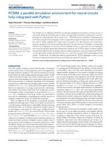
3.2 Servomotor Model Although ODE provides a motor model, a more accurate one was needed in order to simulate the servomotor used in the modules. Thus, a real servomotor model has been developed (Figure 3). This model is built upon the existing motor model provided in ODE library adding a simulation of its parameters. The parameters are as follows: • Kτ[N·m/A] : torque constant • Km[V/rad/s] : counter-electromotive force constant • Kp[V/rad] : proportional servo-control constant • Lm[H] and R[Ω] : electrical parameters of the motor, inductance and resistor • Jm[N·m/rad/s2] : inertia parameter of the motor • Bm[N·m/rad/s] : friction coefficient of the motor And the variables that are used are: • θm[rad] : actual angle (acquired from ODE) • θr[rad] : desired angle • ω[rad/s] : velocity • ea[V ] : voltage of the stator • i[A] : intensity of the current • em[V ] : inducted voltage • τ [N·m] : electromechanical torque of the motor • τloss[N m] : loss of torque due to all intrinsic factors • τeffective[N·m] : effective torque sent to ODE to move the servomotor to the desired position • if [A] : intensity measured after the low pass RC filter used in the real modules to filter the noise. Although it has no purpose in the servomotor model, it is necessary to compare the signal from the real and simulated modules. τeffective can be calculated with the following equations:

��

�� ∙ �� ∙ �� ∙ �� ∙ ��

(1) (2) (3)

Alberto Brunete, Miguel Hernando and Ernesto Gambao: A Simulation Environment for Bio-inspired Heterogeneous Chained Modular Robots

3

Ea must be limited to 5 V, because that is the maximum voltage provided by the power supply. In Figure 3, it is the block before Ea. In the real modules, servomotor control is done by pulse-width modulation (PWM). Param Value

Kp 12

Km 0.14

Kt 0.14

R 12

L 0.0075

B J 35·10-7 7·10-7

specifications of the servomotors of each module. To ensure the proper interaction of the modules with the simulated environment, the friction coefficients were set to the estimated values for possible manufacturing and surface materials. These values were adjusted and validated experimentally in a final step.

Table 1. Parameters for the servomotor tests

(a)

(b)

(c)

(d)

(e)

(f)

(a)

(b) Figure 4. Comparison of the real and simulated servomotors moving from 30º to 120º unloaded. Intensity (a) and torque (b).

There is a range, [0..Ithreshold], where intensity does not produce any torque due to the friction static coefficient. This is represented in Figure 3 with the block before Kt. The optimal parameters found are shown in Table 1. Figure 4 shows a comparison between a real and a simulated servomotor. 3.3 Modules’ Physical Model For better performance and stability, the modules’ model was simplified to a set of standard geometrical primitives (such as spheres, cubes, cylinders, etc.) connected by degrees of freedom (DOF), which were defined as (powered) joints. This simplification of changing odd shapes into standard shapes was necessary to make simulation scalable (collision detection with odd shapes is very expensive in ODE). However, the dimensions and masses’ values were those of the real modules. The geometric morphology model created was then assigned dynamic properties corresponding to the modules’ design specifications. Masses for each body part were assigned real values. The DOFs were limited by the maximum torque and speed available from the

4


Figure 5. Modules: rotation (a), helicoidal (b), support (c), extension (d), touch (e) and traveller (f)

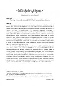
To be capable of producing behaviours with different functionalities, the modules should be able to dock with each other forming different configuration shapes. In the design specification, the modules have two docking faces, one on each side. In the simulated environment, the docking capability was implemented by using a fixed joint that is created by connecting two sides of different modules. This allows the modules to be attached to each other and maintain their relative positions while fixed. All the modules try to maintain similarities with the real ones as much as possible, whether in mechanics (joints, DOF, shape, mass, etc.) or in electronics. Each module model will be described in detail in the following sections. 3.3.1 Rotation Module The rotation module (Figure 5a) is simulated by a capsule and two cylinders as connectors. It has two servomotors that provide the two DOFs and are each limited to 180º as with real servomotors.

Several rotation modules can perform snake-like movements, if sinusoidal movements are applied to their actuators [11]. The following movements have been tested: moving forward and backward, turning, rolling, rotating in place and lateral shifting. 3.3.2 Helicoidal Module The helicoidal module (Figure 5b) is simulated by a pig module (passive), upon which a force is applied in the direction of movement in order to simulate the driving force of the module’s rotating head. This is a simplified model of the real module so as to make simulation faster and less expensive in terms of CPU consumption. The helicoidal module was tested in different slopes with the characteristics shown in Table 2. Angle (◦) Speed (cm/s) (Real) Speed (cm/s) (Simulation)

0 3 3

30 2,1 2,3

60 1,5 1,6

90 1,2 1,3

The inchworm configuration (two support modules and one extension module) was tested as a drive unit. A comparison between the real modules and simulated ones is shown in Table 3. Angle (◦) Speed (cm/s) (Real) Speed (cm/s) (Simulation)

0 2,5 1,5

30 1,5 1,3

90 0,6 0,3

Table 3. Speed test of the inchworm configuration

3.3.5 Touch Module The touch module (Figure 5e) simulates the touch sensor module. The touch sensor is simulated by means of a cylinder that detects collisions. Collision detection is simulated by the detection of contact by the surface of the cylinder (any part) with any other object (i.e., the pipe), something which is quite accurate, because the real module has a cover stuck to three contact sensors; when the cover touches anything, the sensors detect it.

Table 2. Speed test of the helicoidal module

3.3.6 Traveller Module

3.3.3 Support Module

The traveller module (Figure 5f) has been designed to measure the distance travelled by the module. It is composed of three wheels fitted with encoders that measure the distance that the robot has travelled.

The support module (Figure 5c) is simulated by three cubes that represent the arms with three servomotors and two cylinders as connectors. The real module has only one servomotor, but this is an easy way for simulation. One servomotor is the active one, which can be accessed and modified, and the other two simply copy the position of the main one. In order to make the simulation more accurate, passive servomotors should have a smaller torque than the main one, since in the real module there is only one servomotor that sends more torque to one arm than to the other two. 3.3.4 Extension Module

The encoders are simulated by calling a function that gives the rotation (in degrees) of the wheel. The function is provided by ODE API. Since there are three encoders and each of them can measure different distances depending on whether they are in contact with the surface or not, an algorithm is needed to extract an accurate value from the separate ones. This algorithm is embedded in the control program of the module.

The extension module (Figure 5d) is simulated by two cubes that can slide, one over the other, in order to imitate the elongation of the modules. A control has been implemented to simulate a linear servomotor (equations 4 and 5). A circular servomotor in the front can simulate the rotational DOFs of the real module.

The encoders take measurements continuously. At every step of the control algorithm (every 15 ms approx.), it takes a measurement of each of the three encoders and calculates the maximum value. This value adds up to the total value, which is the distance travelled for the module.

(4) (5)

In order to simulate a real wheel fitted with encoders, it is necessary to add some extra friction to the wheels so that they do not keep turning due to inertia. For each wheel, a torque proportional to its angular velocity is applied in the opposite turning direction.

‫ܨ‬௠௔௫ ൌ ‫ܨ‬௠௔௫௦௘௥௩௢ ܸ ൌ ݈଴ ή ሺܲ‫ݏ݋‬௥௘௙ െ ܲ‫ݏ݋‬௦௘௥௩௢ ሻ

Fmaxservo is the maximum force of the servomotor, l0 a proportional coefficient, Posref the desired position, and Posservo the actual position of the linear servomotor.


5

Figure 7. Module Interface

(a)

The real modules are manually attached through male and female connectors. In the simulation, after the modules are created one next to the other, they are attached by creating a fixed joint between them. 3.4 Environment Model

(b)

It is possible to use different environments or surroundings. Pipes, open air and undulated terrains have already been used, and can be seen in Figures 1 (pipe), 5 (open air) and 12 (undulated terrain). Any other terrain or surrounding environment can be used, as long as it is modelled as a mesh object.

(c)

It is desirable to create simulated environments as accurately and as similar to the real world as possible. Physical parameters such as gravity (weights), shapes and pipe dimensions, as well as friction and bouncing coefficients, attempt to imitate those in reality. The interaction of the environment with the modules has been adjusted by means of parameters like soft constraint and constraint force mixing (CFM), error reduction parameter (ERP), friction and bounciness.

Figure 6. Traveller tests: helicoidal (a), snake-like (b) and inchworm (c) configurations

Experiments made with the traveller module inside a pipe show good results, although they can be improved. Figure 6a shows the results when a helicoidal module pushes the traveller module. The results are perfect because now the wheels are in contact with the pipe all the time. Figures 6b and 6c show the results when the traveller module is pushed by the inchworm and snake-like configurations. This time, the results are worse because of the undulated movement and the bumps created in it, which make the wheels lose contact with the surface occasionally. Since the error increases linearly, a possible solution is to use a filter that corrects this displacement for each type of movement. 3.3.7 Common Interface A common interface (Figure 7) has been designed to connect all the modules and allow a bus carrying all the necessary wires and signals to go from one to the other. This electrical bus carries eight wires: two for power (5 V) and ground, two for I2C communication, data (SDA) and clock (SCL), two for the synchronism lines and two for the auxiliary lines (for a video signal, for example).

6


Pipes have been designed in AutoCAD Inventor [7] and then imported into the simulation as tri-dimensional mesh (tri-mesh) objects (with Rheingold 3D [8] and Meshlab [9]). The modules may collide with the pipe, and so it is also possible to define the friction coefficients of the pipe. In addition, the procedure to run the simulation is similar to running the real robot. The modules have to be connected together, attached and then powered up. From that moment onwards, the robot is ready to receive commands or act autonomously. 4. Electronic and Control Simulator 4.1 Software Description The core of the behaviour of every robot is the control algorithm, which determines how the modules coordinate their actions to perform behaviour functionality. In reality, each module has an independent processor running almost identical control programs and exchanging messages through the common bus. However, the physics-based simulation runs on only one computer that executes all the control programs for each simulated module along with solving the dynamics equations. Thus, to achieve realistic results, the

simulation environment has to emulate the concurrent execution of the control programs for different modules and the resulting communication issues. Ideally, this emulation should be micro-processor specific - that is to say, the simulation time of an execution for a particular program instruction should be equivalent to the actual time it takes for the module processors to process that instruction. However, this approach introduces another level of simulation fidelity and, therefore, considerable overhead. It has been decided to follow a simpler route and use concurrency mechanisms provided by the operating system – namely, threads – to emulate simultaneouslyrunning modules. Each simulated module control program has its own independent thread of execution, which runs in an infinite loop. The physics simulation engine spawns all the module threads in the setup routine and then proceeds to the simulation loop. Each module thread yields execution control at the end of its program loop to give control to the simulation thread, which has the highest execution priority. This helps to make simulation smooth and reduce the CPU load. In order to simulate the existence of independent microcontrollers (processors), there are several threads running on the same machine: one thread for each module, one thread for the central control, one thread for the simulation in charge of iterating the world and physical parameters of the modules (i.e., the servos), and one thread for offline genetic algorithm computation (only running when the GA needs to be computed). Emulated concurrency also forces discipline on the control program’s development. The fact that each simulated module runs an independent piece of code requires deep consideration of synchronization and sensor data propagation among the modules in the configuration. Thus, semaphores (critical sections) have been used to protect data that is accessed by several threads at the same time. This realistic approach makes the developed control algorithms much more suitable for transferring them onto real modules, and makes it easier to move the code from the simulation algorithms to the embedded routines running in each module’s microcontroller. The simulator is divided in four parts: a part that is OSdependent and which governs the inputs-outputs (mouse, buttons, messages, etc.); the physics simulation (ODE); the central control; and the control of each module. 4.1.1 Simulation Parameters The main application has a timer that executes two tasks every 20 ms: the simulation loop routine and the drawing functions. The simulation loop routine is in charge of iterating the world of the defined step (usually 0.5 ms).

4.1.2 Optimization Algorithms One of the main objectives of the simulator is to calculate the best configuration of the robot (regarding both module positioning and parameters) for later use in the real robot. Genetic algorithms (GAs) are used for this optimization in two ways: configuration demand and parameter optimization. In configuration demand (in heterogeneous configurations), for a given task the GAs have to determine the modules to be used in order to have an optimal configuration. In parameter optimization, for a given configuration the GAs have to determine the optimum parameters for best performance. This is especially useful in homogeneous configurations, when the robot is performing snake or inchworm movement. GAs are divided into initialization, evaluation, selection, reproduction and termination phases. The evaluation phase uses the simulator to calculate the performance of each individual. 4.2 Actuator Control The position where the servo has to move is normally sent through a PWM signal (from the microcontroller to the servo). In simulation, this is done by simulating the behaviour of the motors as shown in section 3.2. A function with its parameter (the desired position of the servomotor), “setspangle(spangle)”, is used to set motor position: in a real module, this function sends the PWM signal while in the simulator it updates the variable “spangle” that is used by the servomotor as its setting point. 4.3 Sensor Management Sensors are a very important part of the modules and are simulated in different ways, as shown in the following subsections. 4.3.1 Servo Position The servo position sensor is used in many cases to decide whether or not the action is done and which action should be selected next. This sensor is easily implemented by accessing the current state of the modelled servo and retrieving the angle parameter. 4.3.2 Accelerometer A gravity sensor or accelerometer is often used for dynamic locomotion and for detecting abnormal configuration positions. Real modules are equipped with a 3D accelerometer. Its information will be accumulated over time and filtered to determine the direction of acceleration and gravity. Alberto Brunete, Miguel Hernando and Ernesto Gambao: A Simulation Environment for Bio-inspired Heterogeneous Chained Modular Robots

7

I2C is simulated through different C++ classes: message, bus and message queue. In reality, if a message is sent to the bus, it is listened by everybody who is connected to the bus. This is, by definition, because all the modules are connected to the bus and detect differences in wire voltage. However, in the simulation it has to be implemented through a function that sends the message to all the modules connected to the bus.

Figure 8. Accelerometer axis sketch

The accelerometers output a vector [ax,ay,az] showing the direction of the acceleration they are sustaining. From this vector, it is possible to know the orientation. In the simulation, this is simulated by directly accessing the orientation vector of every element of the simulation. When the module is stopped, it is sometimes possible to calculate its orientation from the output of the accelerometers, vector [ax,ay,az]. For example, if the module is in the position shown in Figure 8, the pitch (rotation along the X axis) can be calculated as in eq. 6, and the roll (rotation along the Y axis) as in eq. 7. For the yaw value, extra computation is needed. ௔೤

Ʌ ൌ ௔

೥

௔೥

ɔ ൌ ௔

ೣ

(6) (7)

We are currently considering adding noise to make it more real. 4.3.3 Encoders The traveller module will be equipped with encoders in each of its three wheels in order to evaluate the distance it has travelled.

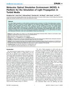
Synchronism lines are used for low-level communication between adjacent modules. It is a kind of peer-to-peer communication, unidirectional in each line. Since there are two lines, communication is bidirectional. Communication along the robot is from module to module, somewhat like passing a baton. Thanks to these lines, every module can be made aware of which other modules are close to it, and the central control of the robot is able to know what the configuration of the robot is. Synchronism lines are connected from the digital output of one module to the digital input of the next. In simulation, two internal module variables - one for the “Sin” signal and one for the “Sout” signal - implement the synchronism line. 4.5 Power Consumption Simulation A model to simulate consumption has been developed following the real design used in the control boards of the modules. This model has been included in the servomotor model, and calculates the current consumed by the motor. It is an experimental model taken from tests with real modules. If the consumption is increasing but the servo is not moving, there is almost certainly a problem (i.e., the servo is stuck). 5. Class Implementation The entire simulation has been built over C++ classes (Figure 9). Each class represents a part of the system. There are classes to simulate the I2C communication protocol (bus, messages, message queue), a class to simulate the servomotor, a class for the whole robot, a general class for a module, a specific class for each module, etc.

This is simulated by a function that reads the rotation of the wheel at regular intervals and calculates how much the wheel has rotated during that time (as in section 2.3.6). When it has the information of all the wheels, this information is processed to compute the distance travelled by the module. 4.4 Communication Simulation Modules can communicate in two ways: using I2C or through two synchronism lines.

8


Figure 9. Class diagram

6. Examples of Use Thanks to the simulator, it is possible to develop movement algorithms for a robot composed of different types of drive modules. The simulator helps to detect problems before the real modules are built, but also helps to detect bad and optimum configurations. It is a test bench where it is easier and faster to test different configurations. Beginning with the locomotion gaits presented in [10-13] and combining them and/or adding other modules, it is possible to obtain better configurations, in the sense of faster, more robust configurations, or configurations able to go to different places. Several examples are given in the following subsections. More examples and detailed information about these configurations and how they are achieved (especially the GA optimization) can be found in [22].

(a) Minimal configuration: contact, rotation and helicoidal

6.1 Minimal Configuration This example shows how the simulator allows for checking the feasibility of the design and predicting its performance. The goal is to identify the minimum number of modules needed in order to use a helicoidal module (because the helicoidal module cannot move by its own means in pipes with elbows). After running the optimization algorithms (shown in 4.1.2) with all possible combinations of all available modules, the result was that the minimal configuration is composed of a contact module, two rotation modules and one helicoidal module (Figure 10a). The robot gets stuck in the pipe when negotiating a bend if only one rotation module is used. Thanks to the optimization algorithm, it is also possible to predict configurations that present the best performance, as shown in the following sections. 6.2 Configuration Demand in a Pipe with an Elbow This experiment was designed to determine the optimum configuration of a robot composed of one touch module and eight rotation or helicoidal modules. The touch module should be in the first position, and the other eight modules can be either rotation or helicoidal modules.

(b) Contact, two rotation, one helicoidal, two rotation and one passive Figure 10. Elbow negotiation

can turn. It is possible to position two consecutive helicoidal modules at the end of the robot because they can turn with the previous rotation module. 6.3 Parameter Optimization in an Undulating Terrain In this experiment, a robot composed of eight rotation modules performed a vertical snake-like motion over an undulating terrain as shown in Figure 12. /The results of the algorithm (whose parameters can be observed in Table IV) are shown in Figure 13. The role of the walls is to prevent the robot from falling to the side. From a population of 40 randomly selected chromosomes, the best individual was obtained in generation 63, corresponding to the following values: 71º amplitude, 14 rad/s angular velocity and 1.36 rad phase. These results show an adjustment to the undulating terrain. The amplitude and angular velocity are related to the peaks and valleys of the undulating terrain.

From a population of 40 randomly selected individuals, the best individual was obtained in generation 17: corresponding to the configuration “THRHRHRHH,” where “T” stands for touch, “H” for helicoidal, and “R” for rotation. The evolution of the GA can be seen in Figure 11. The algorithm results show that the best configuration is the one with the maximum number of helicoidal modules that is able to negotiate the elbow. Helicoidal modules must be placed between rotation modules so that they

Figure 11. Optimization in a pipe with an elbow


9

Figure 12. Example of movement over an undulated terrain

Figure 14. Inchworm configuration

Figure 13. Optimization over an undulated terrain

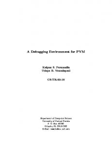
6.4 Several Rotation plus Helicoidal Here, it is possible to detect which is the optimal position for the helicoidal module in the rotation module chain and how many helicoidal modules form the optimal configuration. Figure 10b shows the robot in an exploration task. This includes going forward and negotiating an elbow whenever the contact module detects a bifurcation. The robot is composed of the following modules: one contact, two rotation, one helicoidal, two rotation and one passive. The helicoidal module provides the main drive force. The rotation modules help in going forward with a snake-like movement, but their main task is to turn. 6.5 Several Support plus Several Extension The inchworm gait, usually composed of support + extension + support modules, can be improved by adding more modules (as in Figure 14). Instead of one module of each type, it is possible to set more than one, obtaining the following advantages: • More grip (the grip of one module multiplied by the number of modules), since there are more support modules grasping the pipe. • More speed, because total extension equals the extension produced by one extension module times the number of extension modules. 6.6 Rotation plus Helicoidal plus Support The problem with the helicoidal module is that in order to have grip, all its wheels must be in touch with the pipe. In bifurcations, this is not always possible. Adding the rotation and support modules allows the robot to turn while the support module holds the robot, and the rotation module turns putting the helicoidal module in the next stretch of the pipe to continue moving forward. 10 Int J Adv Robot Syst, 2014, 11:17 | doi: 10.5772/57324

Figure 15. Several rotation, support, extension and helicoidal modules’ configurations

6.7 Several Rotation plus Support plus Extension plus Helicoidal In this combination (see Figure 15), all the locomotion gaits are together: snake-like, worm-like and helicoidal. The robot can change from one to another, depending on the situation. Since the extension module has one rotational DOF, it can take part in some of the snake-like movements. Other modules can act as passive modules in snake-like movements without affecting the overall movement. 7. Conclusion and Future Work In this paper, a simulation environment for heterogeneous chained modular robots has been presented. The simulator has been built upon an existing open source implementation of rigid body dynamics, the Open Dynamics Engine (ODE). Over ODE, a complex system has been built to emulate the behaviour of the robot. An accurate model of the servomotor used by the modules has been built. Modules have been designed to be as simple as possible (using simple primitives) to make simulation fluid, while trying to reflect as much as possible its real physical parameters (mass, torque), leaving aesthetic features in the background. Different

environments (open air and pipes) have been designed, taking into account friction, collisions and interactions between objects. An electronic and control simulator has also been designed. Each simulated module control program has its own independent thread of execution, which runs in an infinite loop. There is another thread for the central control and another one for the GUI. Actuators, sensors communication, (accelerometers, encoders), I2C synchronism lines and power consumption have also been simulated. This simulator has been validated by comparing its results with those obtained from real modules, giving very satisfactory results. It has proven to be a very useful tool for testing configurations and developing prototypes. It helps in obtaining results much faster than with real modules and in avoiding modules breaking during tests. Several examples have been given as to how the simulator can be used to find out new heterogeneous configurations, obtaining interesting results about its locomotion and behaviour. Examples have also shown how the simulator can be used to find specific configurations for a given task (i.e., the minimal configuration for elbow negotiation). An actual limitation of the simulator is the use of simple primitives to simulate the modules. We are currently studying the use of more complex forms to develop a more accurate model of the modules. Future work will also focus on the improvement of the simulator, allowing the user to more easily include new environments and modules. Another goal is to include a window to write directly the code running on the modules and the central control. 8. References [1] http://www.ode.org/ Accessed: 21 Oct 2013 [2] Cortsen, J.; Jorgensen, J.A.; Solvason, D.; Petersen, H.G.; "Simulating Robot Handling of Large Scale Deformable Objects: Manufacturing of Unique Concrete Reinforcement Structures," 2012 IEEE International Conference on Robotics and Automation (ICRA), pp. 3771-3776, 14-18 May 2012 doi: 10.1109/ICRA.2012.6225012 [3] Heinen, M.R.; Osorio, F.S.; "Applying Neural Networks to Control Gait of Simulated Robots, "10th Brazilian Symposium on Neural Networks, 2008, pp. 39-44, 26-30 Oct. 2008. doi: 10.1109/SBRN.2008.22 [4] Jianjun Y., Kang J.; Wentong, G.; "Research on Motion Control of Wheeled Self-balancing Robot Based on ODE Virtual Reality Technology," 2011

Chinese Conference on Control and Decision (CCDC), pp. 2400-2405, 23-25 May 2011 doi: 10.1109/CCDC.2011.5968611 [5] Tanev, I.; Ray, T.; Buller, A.; "Automated Evolutionary Design, Robustness, and Adaptation of Sidewinding Locomotion of a Simulated Snake-like Robot," IEEE Transactions on Robotics, Vol. 21, No. 4, pp. 632- 645, Aug. 2005 doi: 10.1109/TRO.2005.851028 [6] Zlajpah L.; “Robot Simulation for Control Design”, Robot Manipulators Trends and Development, Intech 2010, ISBN: 978-953-307-073-5, InTech [7] http://www.autodesk.com/ Accessed: 21 Oct 2013 [8] http://www.tb-software.com/products_1.html Accessed: 21 Oct 2013 [9] http://meshlab.sourceforge.net/ Accessed: 21 Oct 2013 [10] Choi H.R.; Roh S.G.; “In-pipe Robot with Active Steering Capability for Moving Inside of Pipelines”, Bioinspiration and Robotics Walking and Climbing Robots. Intech 2007, ISBN: 978-3-902613-15-8 [11] Gonzalez, J.; Zhang, H.; Boemo, E.; Zhang, J.; “Locomotion Capabilities of a Modular Robot with Eight Pitch-Yaw-Connecting Modules”, 9th International Conference on Climbing and Walking Robots, Belgium, 2006 [12] Kotay, K.; Rus, D.; “The Inchworm Robot: a MultiFunctional System”, Autonomous Robots, Kluwer Academic Publishers, 2000, Vol. 8, pp. 53-69 [13] Brunete, A.; Torres, J.; Hernando, M.; Gambao, E.; A Proposal for a Multi-drive Heterogeneous Modular Pipe-inspection Micro-robots International Journal of Information Acquisition (IJIA), 2008, Vol. 5, pp. 111-126 [14] http://bulletphysics.org/ Accessed: 21 Oct 2013 [15] http://newtondynamics.com/ Accessed: 21 Oct 2013 [16] Boeing A.; Bräunl T.; “Evaluation of Real-time Physics Simulation Systems”. Proceedings of the 5th International Conference on Computer Graphics and Interactive Techniques in Australia and Southeast Asia (GRAPHITE '07). 2007 ACM, New York, USA, pp. 281-288. DOI=10.1145/1321261.1321312 [17] http://www.cyberbotics.com/overview Accessed: 21 Oct 2013 [18] http://coppeliarobotics.com/ Accessed: 21 Oct 2013 [19] J. C. Zagal, and J. Ruiz del Solar. "UCHILSIM: A Dynamically and Visually Realistic Simulator for the RoboCup Four Legged League". RobuCup, volume 3276 of Lecture Notes in Computer Science, page 3445. Springer, (2004) [20] http://opensimulator.org/ Accessed: 21 Oct 2013 [21] http://gazebosim.org/ Accessed: 21 Oct 2013 [22] Brunete, A.; Hernando, M.; Gambao, E.; "Offline GAbased Optimisation for Heterogeneous Modular Multi-configurable Chained Micro-robots". Transactions on Mechatronics, 2013, Vol. 18, Iss. 2, doi: 10.1109/TMECH.2012.2220560, pp. 578 - 585 [23] http://www.robcib.etsii.upm.es/index.php/en/projects28/micromult Accessed: 21 Oct 2013


11