A Simulation Framework for Evolution on Uneven

A Simulation Framework for Evolution on Uneven Terrains for Synchronous Drive Robot by Aditya Gattupalli, Vijay Eathakota, Arun Kumar Singh, Madhava Krishna

Report No: IIIT/TR/2012/-1

Centre for Robotics International Institute of Information Technology Hyderabad - 500 032, INDIA June 2012

A Simulation Framework for Evolution on Uneven Terrains for Synchronous Drive Robot Aditya Gattupalli, Vijay P. Eathakota, Arun K. Singh, K. Madhava Krishna Robotics Research Centre, International Institute of Information Technology, Hyderabad, [email protected], [email protected], [email protected], [email protected]

Abstract This paper presents a simulation framework for evolution on uneven terrains for a wheeled mobile robot such as a synchronous drive robot. The framework lends itself as a tool capable of solving various problems, such as forward kinematic based evolution, inverse kinematic based evolution, path planning and trajectory tracking. This framework becomes particularly useful when we understand that the evolution problem (and hence the various associated problems based on evolution) is particularly challenging on uneven terrain. Specifically it is entailed to bring in the contact constraints posed by the interaction of the wheel and the ground as well as the holonomic constraints as the problem is formulated in a DAE setting (Differential Algebraic Equation). The problem becomes all the more crucial as vehicles moving on uneven terrain are becoming the order of the day. Nonetheless there has not been much literature that deals in length the various aspects that go into the framework. This paper elaborates on the various aspects of the framework, presents simulation results on uneven terrain, where the vehicle evolves without slipping and also presents substantial quantitative analysis in regard to wheel slippage. The main contributions of this paper are the motion planning using forward kinematic framework and a new formulation of Inverse Kinematics for wheeled robots on uneven terrains.

keywords: Robotic Simulation, Kinematic path planning, Wheeled Mobile Robot

1

Introduction

There have been numerous papers dealing with navigation on uneven terrain [1], [2], [3], [4], [5], [6]. In almost all of these works the problem is formulated as solving for the velocity profile and pose of the platform center as the vehicle navigates on uneven terrain. The corresponding wheel or joint velocities/rates are assumed to exist and readily available when required. However most often as robotic researchers one is required to solve the problem of finding the vehicle evolution given joint velocities. This problem is significantly challenging on uneven terrain wherein the nature of the contact constraints 1

between the wheel and the underlying ground plays a pivotal role in determining the evolution. That apart to ensure the vehicle is in contact with the ground and as well as to avoid numerical integration errors in DAE framework one needs to make sure that holonomic constraints are stabilized during evolution. Such satisfaction of holonomic and contact constraints is not of due concern in evolution in planar terrains, thereby rendering uneven terrain evolution as a significantly unique and challenging problem vis-a-vis planar evolution.

This problem of evolving the vehicle states from the joint rates on uneven terrain has received scant attention in robotic literature, partially because most authors compute pose of the vehicle and joints from sensor feedback having actuated the joints with velocities computed from an inverse Jacobian of platform velocities. This strategy is useful when researchers have real robots to experiment with. In the absence of such real robots, one is entailed to take help of physics engines/dynamic simulation engines like ADAMS and NASTRAN to ascertain the pose and velocity evolution of the vehicle having actuated joint rates/velocities.

The simulation framework proposed and detailed in this paper helps one to bypass the need for experimental testbeds moving on uneven terrain or the requirement of a physics/dynamic simulation engine. Through an elaborate solving of DAE the method computes the forward evolution of any wheeled mobile robot on an uneven terrain. The simulation framework is also a tool that can be used to solve other applications that incorporate uneven terrain evolution as a basic module. Such applications include forward and inverse kinematic based motion planning, trajectory tracking and control. In this paper we show how the framework is used to solve for forward and inverse kinematic based planning for a synchronous drive robot. The detailing of the simulation framework and its application to a syncrho drive evolution and planning constitutes the essential contribution of this work. In a previous effort how forward evolution and planning based on this framework can be accomplished for a Passive Variable Camber (PVC) based Wheeled Mobile Robot (WMR) [7] [8]. In this contribution we go beyond our previous work and depict the generality of the framework by invoking it for the syncrho drive, which is a much more popular and widely used robot than PVC. A forward motion planning algorithm based on the Rapidly Exploring Random Tree(RRT) is developed. An Inverse kinematic framework is developed which the authors believe is a first in uneven terrain navigation. These contributions are elaborated by using the Figures shown below.

In Forward Kinematics usually the platform and the wheel contact velocities are found from the ˙ In most of the cases joint rates are used on Flat terrain and platform centre rates given joint rates Θ. are used in uneven terrains to get the 6-dof vehicle platform posture at each instant as shown in Figure 2 [1], [2], [3], [4], [5], [6]. However these platform evolutions may not be feasible on uneven terrains and may not ensure constraints like no-slip so it is important to consider wheel contact parameters η and joint parameters θ. We use the architecture shown in Figure 1 to evolve the vehicle using Forward 2

Joint Rates for both flat and

˙ Θ

uneven terrain

Forward

6-dof vehicle

Kinematics

platform posture,

solving DAE’s

η,θ

η, θ Current posture

Figure 1: Forward Kinematic Architecture Joint Rates on Flat terrain

˙ Θ

/ Platform

Forward

Vehicle

Kinematics

platform posture

centre rates on uneven terrain

Figure 2: General Forward Kinematics

Kinematics which is in contrast to the general kinematics show in Figure 2. This has been rarely done before as in [9], [10] and in our previous works [7], [8]. But this has not been done for a synchronous drive robot. In our motion planning framework we use the forward kinematic framework shown above and use the algorithm of Rapidly Exploring random tree(RRT) in [11], [12]. Our planning is more robust than the papers cited above as they do not consider the kinematic model and actual wheel contact points of the robot on uneven terrains. From a starting point we give a range of joint rates to find the kinematically feasible evolutions for each joint rate. Then a node closest to the goal is chosen based on the distance metric and the robot proceeds towards the goal iteratively.

Inverse kinematics is generally done by giving suitable platform velocity inputs [Vp ,ωp ] to find out Independent Compute

Inverse Kinemat-

platform

Vp ,ωp

other

ics Framework

velocity components

solving DAE’s

components η, θ

η, θ

6-dof vehicle

Current posture

platform posture, η,θ

Figure 3: Proposed Inverse Kinematic Model

3

Vp ,ωp Platform Velocities

Vehicle J −1

platform posture, ˙ Θ

Figure 4: General Inverse Kinematics

the joint rates and the wheel velocities. This has been done on flat terrain for synchronous drive robot [13] using the platform variables like platform centre co-ordinates and the yaw of the vehicle. These equations perfectly determine the vehicle posture at each interval of time on Flat terrain. However if we really want to ascertain where the robot should evolve given a platform velocity on uneven terrains the computation of wheel contact velocities becomes inevitable. Most methods assume the existence of contact velocities and compute the platform posture as shown in Figure 4. In contrast in this paper we propose an Inverse kinematic module to compute the wheel contact velocities given the platform velocities and further show the evolution of the robot using the simulation framework shown in Figure 3. In our Inverse Kinematic framework we define independent and dependent platform velocity components of a robot and find out the functions connecting the independent and dependent components. The formulation of these precise functions connecting dependent variables to independent variables on uneven terrains has not been done before. These platform velocities are used to get the precise wheel contact velocities using framework developed from dexterous manipulation. Finally these wheel contact velocities are used to get the evolution of the vehicle on uneven terrains. To the best of our knowledge this Inverse Kinematic formulation is unique and has not been done before on any robot.

On a fully 3-D terrain kinematic planning has been a challenging problem. This is especially important in synchro drive vehicles as they are being used frequently for different robotic applications like exploration and mapping on terrains. But a definite theoretical framework for the planning has been lacking on uneven terrains. Earlier works of inverse kinematic formulation in manipulators by Sciavicco and Sciliano [14] and by Han and Trinkle [15] helps in the formulation of the velocity relationships for the synchro drive. Aucther [9] gives a parallel between a Wheeled Mobile Robot and the object manipulator. Using this analogy we derive the Jacobians and the required feasible wheel velocities for the synchro drive. Simulation is done from developing a model of the robot and then giving it appropriate inputs. In this process no multibody simulation software is being used. A set of Ordinary Differential Equations (ODEs) are solved to find the evolution of the wheel ground parameters for the given joint rates. On uneven terrain additional satisfaction of holonomic constraints is required which are not required in flat terrain. As rightfully pointed out in [16], the kinematic analysis on uneven terrain involves solution of a mixed holonomic-nonholonomic set of equations with the characteristics that are distinct from mobile robots on planar/even terrain. This constrained evolution of ODEs is based on the Montana’s Kinematics of contact and Grasp [17] in which the relative evolution of two surfaces with single point of contact is shown. These constraints include kinematic no slip and per4

Methods used

Forward Inverse

and Kine-

matics without

Forward matics

Kine-

Inverse

Kine-

with

matics

with

Motion

Plan-

ning

using

DAE

DAE

DAE

DAE C. Grand et al. [6]

X

×

×

×

M. Tarokh et al. [5]

X

×

×

×

N. Chakraborty et al. [10]

×

X

×

×

K. Iagnemma et al. [3]

X

×

×

×

Proposed method in this

×

X

X

X

paper

Table 1: Comparisions between different methods

manent contact between the wheel and the terrain. To the best of our knowledge on previous works in synchro drive vehicles these constraints were not taken into consideration to get the complete 6-dof kinematic evolution of the vehicle. A comparison of different methods used in uneven terrain navigation is shown in Table 1.

2

Simulation Framework

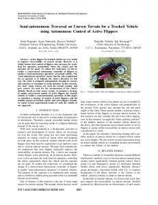
Let us consider a synchronous drive robot on uneven terrain as shown in Figure 10. The robot has 3 degrees of freedom. Given the starting and end goal positions of the robot on uneven terrain we are interested to find a kinematically feasible path that connects these two positions ensuring pure rolling while traversing the terrain. In order to achieve this objective we first develop the kinematics of the robot on uneven terrain for pure rolling constraints. We define the vehicle platform posture as [xp , yp , zp , α, β, γ] where the first three components are the position of the platform and the last three are the euler angles of the platform w.r.t to inertial frames. The platform velocity is defined as [vpx , vpy , vpz , ωpx , ωpy , ωpz ], where the first three represent the linear velocity components while the last three represent the angular velocity components w.r.t to inertial frames.

Forward Kinematics The Forward Kinematics for a three wheeled WMR on uneven terrain shown in the Figure 7 is as follows step1 For a 3-dof robot we give suitable joint rates. From these joint rates and the current posture of the robot wheel velocities and the platform velocities are found out using appropriate jacobian relationships. step 2 The wheel velocities from above are inputs to the montana equations of motion which give us the evolution of the vehicle on uneven terrain. The ODE’s which are solved are constrained with holonomc

5

Figure 5: Torus wheel and ground frame assignments

Figure 6: WMR joints Forward Kinematics using montana and Joint Rates

˙ Θ

dextrous manipulation

xp , yp , zp , α, β, γ

and satisfying

η,θ

holonomic and non holonomic constraints η, θ Current posture

Figure 7: Forward Kinematic Architecture

6

Compute other Independent components platform

vpx ,vpy ,ωpz

using vehicle

velocity geometry and components terrain equation η, θ η, θ Current posture

Inverse Kinematics using montana and Vp ,ωp dextrous manipulation and satisfying holonomic and non holonomic constraints xp , yp , zp , α, β, γ η,θ

Figure 8: Proposed Inverse Kinematic Model

and non holonomic constraints. Solution of this ODE gives us the current posture. Joint rates are smoothly changed with time. Using the current posture and joint rates we iteratively find the remaining dependent platform velocity and wheel velocities in 1 and using these constrained ODE’s are solved in 2 to find the Forward Kinematic motion of the vehicle .

Inverse Kinematics The Inverse motion problem for a three wheeled WMR on uneven terrain shown in the Figure 8 can thus be stated as follows step 1 For a 3-dof vehicle 3 independent components of the platform velocity completely determine its motion. Therefore 3 components of the platform velocity are given as input. We parameterise the platform velocities and find the other components of the platform velocity using the current posture, terrain surface equation and the geometry of the vehicle. step 2 After obtaining the platform velocities using the current posture we find wheel velocities which satisfy the non holonomic constraints using dexterous manipulation framework. step 3 The wheel velocities from above are inputs to the Montana’s equations of motion which give us the evolution of the vehicle on uneven terrain. The ODE’s which are solved are constrained with holonomic and non holonomic constraints. Solution of this ODE gives us the current posture and the joint rates. Velocity components of platform in 1 are smoothly changed with each iteration. Using the current posture we iteratively find the remaining dependent platform velocity components 1, wheel velocities in 2 and using these constrained ODEs are solved in 3 to find the Inverse Kinematic motion of the vehicle .

7

Forward Kinematics Range of

˙i Θ

joint Rates

for each joint rate

Choose the Xj

path closest

as mentioned above

to goal

for certain time η, θ Current posture of the chosen path

Figure 9: Motion Planning Architecture

Figure 10: Synchro drive on uneven terrain

Motion Planning using RRT Forward Kinematics mentioned above is done iteratively for a range of joint rates as shown in the Figure 9. These different joint rates allows the paths to be evolved into Randomly exploring random tree(RRT) as proposed in [11]. ˙ i generate paths from the current posture using the forward step 1 For a range of values of joint rates Θ kinematics problem mentioned above. step 2 Choose the node closest Xj to the goal and repeat the process.

3

Kinematics of the WMR

Definitions : For any two reference frames {A} and {B}, {RAB , PAB } ∈ SE(3) is the transformation matrix of {B} w.r.t {A}, where RAB ∈ SO(3) is the rotation matrix of the frame {B} w.r.t frame {A} and PAB ∈ R3 is the position vector of the origin of frame {B} w.r.t {A}. B The velocity vector of the frame {B} w.r.t {A}expressed in the body frame (VAB ∈ R6 ) is given by

8

   B VAB = 

B υAB

B ωAB

    

(1)

B B T ˆ ˙ Where υAB = RAB P˙AB and ωAB = RAB RAB , ˆ operator extracts the vector associated with the skew

symmetric matrix. For any three reference frames {A}, {B} and {C} we have C B C VAC = Ad−1 BC VAB + VBC

(2)

Where the adjoint transformation matrix and its corresponding inverse between frames {A} and {B} is given by  AdAB = 

RAB 03×3

ˆ RAB PAB RAB





 , Ad−1 =  AB

T RAB

T ˆ −RAB PAB

03×3

T RAB

 

Frame Assignments : Figures 10 and 5 show the details of the frame assignments we have considered in our analysis. {G} is the frame assigned to the ground frame, {P } is the frame fixed at the center of mass of the platform. {CGi } is the frame fixed on the ground, at the contact point of the ith wheel with the ground. {Wi } is the frame assigned to the center of the ith wheel and {CWi } is the frame fixed on the wheel at the contact point. ψi is the angle between xCGi and xCWi . As can be seen from Figure 6 all the three wheels are steerable and the angle of steer is given by φi ∀i = {1, 2, 3}. αi ,∀i = {1, 2, 3} is the angle of rotation of the wheels about the ZWi axis.

3.1

Montana’s kinematics of contact

Let [uwi , vwi , fw (uwi , vwi )]T be the parameterization of the contact point on the torus wheel with the ground and [ugi , vgi , fg (ugi , vgi )]T be the parameterization of the contact point on the ground with the wheel. Also let {Mg , Kg , Tg } and {Mwi , Kwi , Twi } be the metric, curvature and the torsion forms of the ground and the ith wheel respectively. vxi , vyi , vzi , ωxi , ωyi , ωzi are the velocities of it h wheel centre w.r.t ground. Then the variation of the vxi , vyi , vzi , ωxi , ωyi , ωzi given by inverse of Montana’s kinematic equations of contact [17]. 

vxi



vyi





 = −Mwi 



ωyi



−ωxi

uw ˙i vw˙ i





 + rψi Mg  

 = −Kwi Mwi  

ωzi = ψ˙i − Twi Mwi 



uw ˙i vw˙ i

uw ˙i vw˙ i 

u˙gi v˙gi



  

 + rψi Kg Mg  

 − Tg Mg 

u˙gi v˙gi

u˙gi v˙gi

 

 

vzi = 0  Where rψi = 

cos ψi

− sin ψi

− sin ψi

− cos ψi

(3)   is the 2D representation of the frame {CWi } w.r.t {CGi }.

9

For pure rolling we have 

vxi



vyi

 =0

(4)

The constraint that ensures that the wheel does not leave the contact with the terrain is given by vzi = 0

(5)

The constraints for pure sliding is given by 

ωxi



   i   ωy  = 0   i ωz

(6)

Velocity relationships:We assume all the velocities expressed in the body frame unless otherwise stated. For the ith kinematic chain we have.  T˙GP = 

R˙ GP

P˙GP

0

0

 



VP G

 P˙GP  = ˙ RP Gˆ.RGP

(7)

where the first three are the linear components and the last three are the angular components of the platform velocity. We can represent platform velocities in terms of wheel ground parameters and joint parameters as   θ˙  VP G = ΦVP  (8) η˙ where ΦVP are the coefficients extracted for joint parameters θ˙ and wheel ground contact parameters η˙ Also VP Wi is given by VPWWi i = JP Wi (θi )θ˙i

(9)

Where JP Wi is the Jacobian between the platform frame {P } and the center wheel {Wi } and θ˙i is h iT the corresponding joint rate of the ith kinematic chain. Also we have θ˙i = φ˙i α˙i ∀i = 1, 2, 3 The robot jacobian combines these for all the wheels    JR =  

JP W1

0

0

0

JP W2

0

0

0

JP W3

    

VCGi CWi represents the relative velocities of the contact frames {CWi } w.r.t {CGi } ∀i = 1, 2, 3 . in the h iT CW respective body frames. We represent this velocity vector as VCG iCW = vxi vyi vzi ωxi ωyi ωzi i i CW

CWi C i Wi

From Montana’s kinematic equations of contact we have VGWii = VCG Wi VPWGi = VW + VPWWi i iG

10

(10)

CW

AdWi G VPGG + AdWi CWi VGWii = JP Wi θ˙i

(11)

Augmenting equation (11) for all wheels we form the following Jacobian which relates the joint rates of the robot to the platform velocity and the wheel- ground contact velocity which is written as     VPGG   AdW1 G AdW1 CW1 0 0 CW1     V   GW1   = JR θ˙   CW   AdW2 G 0 AdW2 CW2 0  V 2    GW2 AdW3 G 0 0 AdW3 CW3  CW  VGW33 JGC VGC = JR θ˙

(12)

(13)

where JGC is the matrix consisting of Adjoint matrices and VGC is the augmentation of platform and wheel ground contact velocities. Equation (13) represents the non holonomic constraints of the system.

3.2

Synchro and Holonomic constraints

The closed loop kinematic chains give rise to a set of constraints know as the holonomic constraints on the robot and ground parameters which can be written as. {RP G , PP G }W1

−

{RP G , PP G }W2 = 0

{RP G , PP G }W1

−

{RP G , PP G }W3 = 0

(14)

These set of algebraic constraints of the form H(Θ) = 0 can be differentiated to a set of ODEs of the form ˙ + σH(Θ) = 0 J(Θ)Θ

(15)

where Θ is the set of Wheel ground parameters and Robot Joint angles. The above method of convergence of constraints is mentioned in [18]. In addition to these constraints we also have a constraint on the steer of three wheels which have to be same at each instance.

 

φ1 − φ2 φ1 − φ3

 =0

(16)

The above two constraints L(φ) = 0 are differentiated to form set of ODEs of form K(φ)φ˙ + σL(φ) = 0

3.3

(17)

Forward kinematic Equations of the Robot

Forward kinematics of the robot involves solving for the Robot’s position and velocities given the desired joint rates. To get the desired velocities from the joint rates (13) is used. + VGC = JGC JR θ˙

11

(18)

+ where JGC is the pseudo inverse of JGC

We get the equations for the wheel velocities from (18). In this equation joint rates are smoothly changed over time. These are used to solve the set of ODEs by incorporating (15) and (17) in (3) ∀i = {1, 2, 3} . These ODEs are integrated at each step along with the integration of the joint rates to get the evolution of the robot using forward kinematics formulation.

3.4

Inverse kinematic Equations of the Robot

Inverse kinematics of a mobile robot involves solving for the wheel velocities given the platform velocity. For a WMR traversing on an uneven terrain all six components of the platform centre exists. They are [vpx , vpy , vpz , ωpx , ωpy , ωpz ], where the first three represent the linear velocity components while the last ˙ γ), ˙ γ) three represent the angular velocity components.We know that ωpx = g1 (α, ˙ β, ˙ ωpy = g2 (α, ˙ β, ˙ and ˙ γ) ωpz = g3 (α, ˙ β, ˙ where α, β, γ are yaw, roll and pitch of the robot. However only vpx , vpy and α˙ can be controlled for a passive or Rigid suspension WMR. We will refer to these as the active variables. The objective is to estimate the six components platform velocity in terms of the active varaibles. For that we need functions of the form β˙ = h1 (vpx , vpy , α), ˙ γ˙ = h2 (vpx , vpy , α) ˙ and vpz = h3 (vpx , vpy , α), ˙ which is derived in the following manner using the holonomic constraint describing the geometry of the vehicle

PP G + PGCwi = PP Cwi PGCwi = RGP [δ1i W

where

δ1i

0 i=1 = −1 i = 2 1 i=3

δ2i L

and

(19)

− H]T

δ2i

=

(20)

−2 1

i=1 i = 2, 3

and W, L and H describe the vehicle geometry as shown in the Figure 10 The equations of wheel ground contact points xCwi , yCwi , zCwi corresponding to ith wheel computed using (20) are xCwi = xp − δ2i Lsin(α) − δ1i W cos(α) − Hγsin(α) − Hβcos(α)

(21)

yCwi = yp + δ2i Lcos(α) − δ1i W sin(α) + Hγcos(α) − Hβsin(α)

(22)

zCwi = zp + δ2i Lγ + δ1i W β − H

(23)

The terrain equation is then linearised around platform centre.

zCwi = k3 + k2 (xCwi − xp ) + k1 (yCwi − yp ) where k1 =

∂fg ∂ug |ug =xp ,vg =yp ,

k2 =

12

∂fg ∂vg |ug =xp ,vg =yp ,

k3 = fg (xp , yp )

(24)

Here fg is the function of parameterisation of the ground point mentioned in section 3.1. This linearisation is justified since any terrain can be locally represented by a linear plane having a particular orientation in 3D space. By incorporating equations (21), (22) and (23) in (24) we get a matrix of the form



1

   1  1

A11 A21 A31

A12



zp





B1



        A22   γ  =  B2      B3 β A32

(25)

Where the coefficients of the matrix are the coefficients of equation (24) corresponding to three wheels. All the coefficients are in xp , yp , α. So by inverting the matrix we can get the values of zp , γ and β in terms of them. Then by differentiating the equations for zp , γ and β we get differential components of them. This will be used to get the desired velocity of the platform VP Gd . From (13) a QR matrix decomposition is performed on JR JR = QR

(26)

Q is split into [Q1 Q2 ] where Q2 forms the orthogonal basis of JR T .Hence DVGC VGC = Q2 T JGC VGC = 0

(27)

Again taking QR decomposition of DVGC we get [QV1 QV2 ]RV . After few elementary transformations we get VGC in terms of the desired VGCd as VGC = QV2 QTV2 VGCd

(28)

These set of velocities satisfy the non holonomic constraints mentioned in (13). The equations (3),(8) ∀i = {1, 2, 3} , (15) and (17) form a set of ODEs which represent the Inverse kinematic relationships of the WMR on uneven terrain. The inputs to these equations are the platform and wheel velocities found in (28). The inputs of linear wheel velocities are set to zero as mentioned in (4) to ensure pure rolling. These set of equations can be integrated numerically to get the configuration parameters of the system at each time instant.

3.5

Motion Planning using Forward Kinematics

We develop a Motion Planning algorithm for the WMR on uneven terrain. Planning algorithm is based on Rapidly Exploring Random trees(RRT) as in [11], [12]. The paths between adjacent nodes of the RRT are generated using the forward Kinematics problem formulated above. RRT is advantageous as no a priori knowledge of the environment is required. From the current position using the distance metric we determine the node which is closest to the goal and then take this as our new position. The tree constructed in RRT incrementally reduces the distance of the goal to the current tree node. Xj+1 = Min((xpi,j − xpg )2 + (ypi,j − ypg )2 + (zpi,j − zpg )2 ) i

13

(29)

Figure 11: Snapshots of the WMR on Uneven Terrain

where xpg , ypg and zpg represent the goal position of the robot and xpi,j , ypi,j and zpi,j represent the position of the robot at the ith choice of joint rates at the j th iteration. Equation (29) describes the next state Xj+1 of the robot from the available i choices of the joint rate in the Xj state. This will be based on the minimum distance metric used in (29). Thus the robot will reach its goal from the starting point after few iterations.

4

Results and Discussion

In the results we present we use a synchronous drive robot with the following dimensions , Width W = 0.5m, Height H = 0.65m and Length L = 0.33m shown in the Figure 10. The radius of the torus tube R1 = 0.05 m and the distance from the centre of the tube to the centre of the torus is R2 = 0.25m. The terrain used should be continuous and differentiable at each point for which any spline curves can be used. For our simulation we are using product of two sine functions as our terrain where x=ug , y= vg and z=fg (ug , vg ).

4.1

Results of Forward Kinematics

We show the results of the synchro drive robots using Forward kinematic architecture on uneven terrain. This terrain has variable curvature and torsion in each direction. The set of ODEs mentioned in Forward Kinematics section are solved using ODE45 solver in MATLAB. Figure 11 shows the snapshots of the vehicle as it moves on the terrain. In this Figure 11 we can clearly see the path of the three wheels on terrain. Corresponding to this path the Figures 13a and 13b give the L2 norm of the synchro and holonomic constraints which can be seen to be very low (10−3 ) indicating the satisfaction of these constraints. Figures 12a and 12b give us the Linear and the Angular platform velocities respectively. The Linear and Angular velocities can be seen to be varying smoothly over time which indicates the satisfaction of the non holonomic constraints.

14

Angular Velocity of platform Angular Velocities of the Platform in rad/s

Linear Velocity of platform Linear Velocities of the Platform in m/s

0.6 Vpx Vpy

0.4

Vpz

0.2

0

−0.2

−0.4

−0.6

−0.8 0

20

40

60

80

100

120

140

160

180

200

0.08

ωpx ωpy

0.06

ωpz

0.04

0.02

0

−0.02

−0.04

−0.06 0

20

40

60

80

100

120

140

160

180

200

Time in seconds

Time in seconds

(a) Linear Velocity

(b) Angular velocity

Figure 12: Linear and Angular Velocity of the platform

4.2

Results of Inverse Kinematics

We show the results of the synchro drive robots using Proposed Inverse kinematics model on uneven terrain. This terrain has variable curvature and torsion in each direction. The set of ODEs mentioned in Inverse kinematics section are solved using ODE45 solver in MATLAB. We show along one path the snapshots of the vehicle as it moves on the terrain Figure 14. The heading of the vehicle is showed on the platform as a black line in Figure 14 which shows that the vehicle heading is same irrespective of the steering angles of the wheels thus confirming the synchronous drive model. Corresponding to this path the Figures 17a and 17b give the L2 norm of the synchro and holonomic constraints which can be seen to be very low (10−3 ) indicating the satisfaction of these constraints. Figures 15a and 15b give us the input Linear and the Angular platform velocities respectively (VP GD ). The inputs vpx , vpy are smooth sinusoids and ωpz is 0.01rad/s. The other dependent velocity components can be seen to be smoothly varying in Figures 15a and 15b. The input velocities in Figures 15a and 15b are transformed using (28) to get a feasible set of velocities that we show in Figures 16a and 16a. Contact wheel velocities found from the platform velocities are shown in Figures 19b, 20a and 20b. These will be used as inputs to the ODE mentioned in above section. The Figures 18a, 18b and 19a indicates the slip velocities of three wheels from which we can clearly see that the robot is traversing the terrain without any slip.

4.3

Results of Motion Planning

RRT is generated using the forward kinematics and is shown in Figure 21. The figure shows the evolution of the front wheel for a range of joint rates from a common starting position. The tree is spread using 2 goal positions from the same initial position of the robot. Each iteration the robot is given a range of joint rates and is evolved. Then it chooses the path which is closest to the goal from the available choices and moves towards the goal as shown in Figure 21. Path towards goal1 is shown in black and the constraint satisfaction of that path is shown in Figures 22a and 22b

15

Synchro constraint stabilisation

−3

10

x 10

Holonomic Constraint Stabilization 0.04

φ1 − φ2 φ1 − φ3

0.035

6

0.03

L Norm C(q)

4 2

0.025 0.02

2

Synchro constraint L(φ)

8

0

0.015

−2

0.01

−4

0.005

−6 0

20

40

60

80

100

120

140

160

180

0 0

200

20

40

60

80

100

120

140

160

180

200

Iteration

Iteration

(a) Synchro Constraints

(b) Holonomic Constraints

Figure 13: Synchro and Holonomic Constraint Stabilization

Figure 14: Snapshots of the WMR on Uneven Terrain

Linear velocities of the platform Linear velocities of the platform in m/s

Angular velocities of the platform in rad/s

Angular velocities of the platform

8

vdpx vdpy

6

vdpz 4 2 0 −2 −4 −6 −8 0

20

40

60

80

100

120

140

160

180

200

Iteration

1

ωpx ωpy

0.8

ωpz

0.6 0.4 0.2 0 −0.2 −0.4 −0.6 −0.8 −1 0

20

40

60

80

100

120

140

Iteration

(a) Linear Velocity

(b) Angular Velocity

Figure 15: Linear and Angular Velocity of the platform

16

160

180

200

Angular velocities of the platform after transformation in rad/s

Linear velocities of the platform after transformation in m/s

Linear velocities of the platform after transformation 0.5

vpx vpy

0.4

vpz

0.3 0.2 0.1 0 −0.1 −0.2 −0.3 −0.4 −0.5 0

20

40

60

80

100

120

140

160

180

200

Iteration

Angular velocities of the platform after transformation 0.05

ωpx ω

0.04

py

ωpz

0.03 0.02 0.01 0 −0.01 −0.02 −0.03 −0.04 −0.05 0

20

40

60

80

100

120

140

160

180

200

Iteration

(a) Linear Velocity

(b) Angular Velocity

Figure 16: Feasible Linear and Angular Velocity of the platform

Synchro constraint stabilisation

Holonomic Constraint Stabilization

0.01

0.014

φ1−φ2

0.012

L Norm H(Θ)

0.01 0

0.008

0.006

2

−0.005

0.004 −0.01 0.002

−0.015 0

20

40

60

80

100

120

140

160

180

0 0

200

20

40

60

80

Iteration

100

120

140

160

180

200

Iteration

(a) Synchro Constraints

(b) Holonomic Constraints

Figure 17: Synchro and Holonomic Constraint Stabilization

Slip velocities of first wheel

−3

x 10

v1y

2

1.5

1

0.5

0

−0.5 0

20

40

60

80

100

120

140

Slip velocities of second wheel

−3

2.5

v1x

Slip velocities of second wheel in m/s

2.5

Slip velocities of first wheel in m/s

Synchro Constraint L(φ)

φ1−φ3 0.005

160

180

x 10

v2y

2

1.5

1

0.5

0

−0.5 0

200

Iteration

v2x

20

40

60

80

100

120

140

160

Iteration

(a) Slip velocities of wheel one

(b) Slip velocities of wheel two

Figure 18: Slip Velocities of wheels one and two

17

180

200

Slip velocities of third wheel

−3

x 10

Contact velocities of Wheel one 0.6

v3x v3y

2

ω1x ω1y

0.4

Contact velocities in rad/s

Slip velocities of third wheel in m/s

2.5

1.5

1

0.5

ω1z

0.2 0 −0.2 −0.4 −0.6 −0.8

0 −1 −0.5 0

20

40

60

80

100

120

140

160

180

−1.2 0

200

20

40

60

80

Iteration

100

120

140

160

180

200

Iteration

(a) Slip velocities of wheel three

(b) Contact velocities of wheel one

Figure 19: Slip Velocities of three wheels and Contact velocities of wheel one

Contact velocities of Wheel two

Contact velocities of Wheel three

0.8 0.6

ω2y ω2z

0.4 0.2 0 −0.2 −0.4 −0.6 −0.8

ω3y ω3z

0 −0.2 −0.4 −0.6 −0.8 −1

−1 −1.2 0

ω3x

0.2

Contact velocities in rad/s

Contact velocities in rad/s

0.4

ω2x

20

40

60

80

100

120

140

160

180

−1.2 0

200

Iteration

20

40

60

80

100

120

140

160

180

Iteration

(a) Contact velocities of wheel two

(b) Contact velocities of wheel three

Figure 20: Contact wheel velocities of wheel two and three

Figure 21: RRT algorithm over forward kinematics

18

200

Holonomic Constraint Stabilization

Synchro constraint stabilisation

0.045

0.015

φ1−φ2 φ1−φ3

0.04 0.01

Synchro constraint L(φ)

L2 Norm C(q)

0.035 0.03 0.025 0.02 0.015 0.01

0.005

0

−0.005

−0.01 0.005 0 0

50

100

150

200

−0.015 0

250

Iteration

50

100

150

200

250

Iteration

(a) Holonomic constraints

(b) Synchro constraints

Figure 22: Constraint stabilisation of the RRT path to goal1

5

Conclusions

The paper presented a method to simulate Wheeled Mobile Robots(WMR) on uneven terrain using kinematic framework. Simulation is done for a popular synchro drive robot. Along with this the formulation made sure the satisfaction of holonomic and non-holonomic constraints, synchro drive constraints, permanent contact constraints and kinematic no slip at every instant of the evolution. A novel method to calculate wheel contact velocities from the independent platform velocity components is shown in Inverse kinematics. The authors believe that this is possibly the first such effort that provides for the satisfaction of all the above constraints to get the precise 6-dof evolution of paths using both forward and inverse kinematics on an uneven terrain as previous methods of kinematics do not deal with the evolution of wheel ground contacts using DAE’s. Most previous methods have either approximated the process of predicting the vehicle evolution or simplified assumptions of the terrain geometry or evaluated the satisfaction of constraints as a decoupled post-processing step from the vehicle evolution framework. This formulation can be used to simulate number of other Robots using different steering mechanisms and having different degrees of freedom.

REFERENCES [1] T. Howard and A. Kelly, ”Trajectory Generation on Rough Terrain Considering Actuator Dynamics.” Proceedings of the 5th International Conference on Field and Service Robotics,(July 2005) [2] J.V. Mir´ o , G. Dumonteil , C. Beck. , G. Dissanayake. ”A kyno-dynamic metric to plan stable paths over uneven terrain.” IEEE/RSJ International Conference on Intelligent Robots and Systems, pp. 294-299, (2011) [3] G. Ishigami, G. Kewlani, K. Iagnemma, ”Statistical mobility prediction for planetary surface exploration rovers in uncertain terrain.” IEEE International Conference on Robotics and Automation, pp. 588-593, (2010) 19

[4] Z. Shiller and Y.R.Gwo, ”Dynamic motion planning of autonomous vehicles.” Robotics and Automation, IEEE Transactions on,Vol. 7,No. 2,pp. 241-249,(1991) [5] M Tarokh and G.J. McDermott ,”Kinematics Modeling and Analyses of Articulated Rovers.” Robotics, IEEE Transactions on , Vol. 21, No.4, pp. 539- 553,(2005) [6] C. Grand, F. BenAmar, and F. Plumet, ”Motion kinematics analysis of wheeled-legged rover over 3d surface with posture adaptation.” IFToMM world congress, (2007) [7] Vijay Eathakota, Gattupalli Aditya, Madhava Krishna , ”Quasi-static motion planning on uneven terrain for a wheeled mobile robot.” IEEE/RSJ International Conference on Intelligent Robots and Systems, pp. 4314-4320, (2011) [8] Vijay Eathakota, Gattupalli Aditya , Madhava Krishna, ”Quasi-Static Simulation of a Wheeled Mobile Robot having a Passive Variable Camber.” IFToMM world congress, (June 2011) [9] Joseph Auchter and Carl Moore., ”Off-Road Robot Modeling with Dextrous Manipulation Kinematics.” IEEE International Conference on Robotics and Automation,pp 2313-2318, (May 2008) [10] N. Chakraborty, A. Ghosal, ”Kinematics of wheeled mobile robots on uneven terrain.” Mechanism and machine theory,Vol. 39, No.12, pp. 1273-1287, (2004) [11] Steven M. Lavalle, James J.Kuffer Jr., ”Randomized Kinodynamic Planning”, International Journal of Robotics Research, Vol. 20, No. 5, pp. 378-400, (May 2001) [12] A. Ettlin and H. Bleuler, ”Randomised rough-terrain robot motion planning” IEEE/RSJ International Conference on Intelligent Robots and Systems,pp. 5798-5803, (2006) [13] Y. Zhao and S.L. Bement , ”Kinematics, dynamics and control of wheeled mobile robots.” IEEE International Conference on Robotics and Automation,pp. 91-96, (1992) [14] L. Sciavicco and B. Siciliano , ”A solution algorithm to the inverse kinematic problem for redundant manipulators.” IEEE Journal of Robotics and Automation,Vol. 4, No. 4, pp. 403-410, (1988) [15] L. Han and J.C. Trinkle , ”The instantaneous kinematics of manipulation.” IEEE International Conference on Robotics and Automation,Vol. 3,pp. 1944-1949, (1998) [16] B.J. Choi and S.V. Sreenivasan, ”Gross Motion Characteristics of Articulated Mobile Robots with Pure Rolling Capability on smooth uneven surfaces.” IEEE Transactions on Robotics and Automation, Vol. 15, No.2,pp. 340-343 (April 1999) [17] D.J. Montana, ”The kinematics of multi-fingered manipulation.” Robotics and Automation, IEEE Transactions on,Vol. 11, No.4, pp. 491-503,(1995) [18] J Baumgarte , ”A new method of stabilization for holonomic constraints.” Journal of Applied Mechanics,Vol. 50,pp. 869,(1983)

20