Jul 8, 2003 - interference (e.g., power-line noise) and baseline wander as in [1]. However, ... ditional reference channels for carrying out noise cancellation.
A Single-Lead ECG Enhancement Algorithm using a Regularized Data-Driven Filter
Xiao Hu a , Valeriy Nenov b a Biomedical
Engineering Interdepartmental Program, University of California, Los Angeles, CA 90095
b Division
of Neurosurgery, School of Medicine, University of California, Los Angeles, CA 90095
Abstract The present work improves the subspace filter as Electrocardiogram (ECG) enhancer for removing Electromyogram (EMG) contaminations. A unified view of the data matrix formulation process of the existing subspace filters was achieved by considering an enhancement problem as a parameter estimation problem of a linear empirical generation model of ECG. In contrary to a linear prediction (LP) model implicitly assumed in the conventional subspace filters for ECG enhancement, a multiple cycle prediction (MCP) model was proposed, which resulted in a data matrix that is more suitable for applying the truncated singular value regularization technique to parameter estimation. As a necessary step for building an MCP, alignment of two ECG cycles with different length was handled by a dynamic time warping (DTW) algorithm. Finally, the separation of the signal and noise subspaces was realized by a run-time singular value decomposition (RTSVD). RTSVD provides an automatic and adaptive way of determining the dimension of the signal subspace. Representative records from the MIT-BIH Arrythmia Database were combined with EMG noise in the MIT-BIH Noise Stress Test Database with a a typ-
Preprint submitted to Elsevier Science
8 July 2003
ical 10dB signal-to-noise ratio for which the proposed method achieved about 5dB boost while it achieved about 10dB boost for the EMG recorded in our experiment. Key words: Electrocardiogram, Subspace filter, Singular value decomposition, PhysioNet PACS:
1
Introduction
ECG signals collected in such adverse situations as during exercises, and stress tests are often contaminated by EMG signals whose spectrum overlaps that of ECG. This makes the conventional ECG enhancement methods based on finite impulse response (FIR) filter or infinite impulse response (IIR) filter useless without introducing significant distortions of the original ECG. Various more sophisticated and capable ECG enhancement methods have been proposed. Adaptive filters have been shown as highly effective in removing narrow-band interference (e.g., power-line noise) and baseline wander as in [1]. However, their success in ECG enhancement has been limited by the requirement of additional reference channels for carrying out noise cancellation. A category of methods without such limitations has recently been proposed. These methods share the same main idea that a noisy ECG can be enhanced by its projection onto a proper signal subspace but they are quite different in the way they formulate such a signal subspace. In situations where a multiple-lead ECG is available the method [2] worked by exploiting the redundancy of the multiple channels where the signal subspace is revealed by a singular value decomposition (SVD) of a data matrix formed straightforwardly from the 2-dimensional (time and channel) recordings. In more general situations of a single-lead ECG, 2
methods proposed in [3], and [4] formulated a data matrix in the discrete cosine transform domain from which SVD was applied for constructing a signal subspace. SVD technique was also used in [5] for extracting fetal ECG from a single maternal ECG where the data matrix for forming signal subspace was constructed by arranging cycles of maternal ECG in consecutive rows. In another method proposed in [6], the formation of the data matrix was based on the embedding theory developed in the field of nonlinear dynamic analysis of time series and a nearest neighbor search procedure in the embedded statespace. An array of such methods (called geometric filters) has been extensively discussed in [7], [8], and [9]. The present work aimed at further developing the subspace filters as ECG enhancer by first providing a unified view of the aforementioned subspace filters and then exploring a widely used alignment algorithm in speech signal processing, i.e., the dynamic time warping (DTW) for aligning different ECG beats. The alignment of ECG beats is a necessary step for properly formulating the data matrix on which subspace decomposition is carried on. Finally, we propose a run-time SVD algorithm which exploits the morphology of ECG for an automatic and adaptive signal subspace dimension determination. We are able to achieve a unified view of the various subspace filters by considering the data matrix formulation process as formulating an empirical signal generation model which will lead an enhancement problem to a model parameter estimation one in a typical noise-in-variable scenario. By proceeding in this way, the solution space for the enhancement problem is enlarged since projecting a noisy signal onto a signal subspace is equivalent to a truncated SVD which is just of one of regularization techniques for solving noise-in-variable parameter estimation problems as discussed in [10]. 3
A multiple cycle prediction (MCP) model is proposed for modelling ECG generation in this paper which requires an alignment of previous cycles of ECG to the current one. This step is also required in many existing algorithms [5,11] that exploit the quasi-periodic nature of ECG. However, techniques used so far are either linear stretch or a zero-padding one. The major problem of a rigid linear stretching is that such a method cannot handle a very common phenomenon of ECG that cycle duration is not proportional to the width of characteristic waves. Zero padding is just an arbitrary procedure for convenience without any justification. DTW avoids these limitations by performing a nonlinear stretching such that different characteristic waves present in each ECG cycle can be aligned simultaneously.
Finally, determining a proper dimension for the signal subspace is a difficult problem. Some general algorithms have been proposed in the context of rank determination [12]. There is no automatic and systematic way of performing such a task as in the existing subspace-based ECG enhancement algorithms. Furthermore, signal dimension may be a changing number within one ECG cycle since QRS, P and T waves have both different morphologies and amplitudes. Therefore, ideally an adaptive way of dimension determination should be preferred. For such a purpose, we propose a run-time SVD algorithm which slides a window across an ECG cycle and thus a different signal subspace dimension can be automatically determined for each window.
Throughout the text, a boldface lower case letter is used to represent a vector. An upper case letter represents a matrix. Any letter with the additional symbol ”˜” on top represents its perturbed version and its estimate with the symbol ”ˆ”. 4
2
Methods
2.1 Problem formulation
In this section, an empirical signal generation model is proposed based on which the ECG enhancement is to be viewed as a parameter estimation problem. Before proposing such a model, the problem of regularizing linear leastsquare solutions will be discussed. Then it can be shown that the truncated singular value decomposition is just one of many techniques of conducting regularization. The empirical signal generation models that we are interested in using for ECG enhancement are linear ones such that all of them can be eventually reduced to the following common form: x = Hb
(1)
where x denotes a signal vector that is a linear function of unknown parameter vector b, and H is a data matrix that is considered as known. Now suppose we have an observation of x which has an additive observation noise v such that x ˜ = Hb + v
(2)
The enhancement problem is to recover as much as possible x from x ˜. As a classical result for linear models, the maximum likelihood (ML) estimate of b ˆ ml . This implies that given x ˜ will also give a ML estimate of x, i.e., x ˆ ml = H b an enhancement problem is closely related to parameter estimation problem. 5
However, a more difficult and realistic problem is that although H is known, it is also contaminated by noise such that the model reads now as ˜ +v x ˜ ≈ Hb
(3)
In this case, although a ML estimate of b might not guarantee a ML estimate ˆ to of the x, it can achieve certain amount of noise reduction by applying b ˜ to retrieve x. In doing so, the enhancement problem becomes a problem of H ˆ which is a well known noise-in-variable estimation problem (since finding b, H is also contaminated). The ordinary least squares (OLS) solution is not anymore an appropriate one for such a problem, nevertheless it serves as a good starting point for motivating the idea of regularization. This is achieved ˜ by formulating the OLS solution in terms of the SVD of H ˜ M ×N = U˜M ×M Σ ˜ M ×N V˜NT×N H
(4)
˜ are called singular where the diagonal entries σ ˜i , i = 1, . . . , min(M, N ), of Σ values and are ordered with decreasing magnitude. The minimal norm OLS solution of b is ˆ ols = b
r X ˜ T U˜i x i=1
σ ˜i
V˜i
(5)
˜ which is less or equal to the number of non-zero where r is the rank of H, σ ˜i s. As σi decreases with increasing i, V˜i becomes more fluctuating. Hence, ˜ T U˜i is slower than Equation 5 clearly reveals that as long as the decay of x σ ˜i with increasing i, more and more fast components will enter the solution. This is not desirable for our purpose of ECG enhancement since high-frequency portion of the ECG spectrum is usually dominated by EMG. 6
As a remedy to such a problem, the technique of regularization [10] is to find an appropriate set of ”filtering” coefficients fi such that the estimate of b is obtained as ˆ= b
r X i=1
fi
˜ T U˜i ˜ x Vi σ ˜i
(6)
Usually, fi is a non-increasing series aimed at dampening small singular values. One way of choosing fi is to keep first d greatest singular values in the reconstruction equation as in Eq.6, equivalently f = [1, . . ., 0 . . .]. This resulted in | {z } d
the widely used truncated SVD (TSVD) algorithm as employed in other subspace filtering algorithms of ECG. There are two categories of regularization methods. TSVD belongs to the non-iterative group to which other methods such as Tikhonov regularization, damped SVD, and maximum entropy regularization etc. also belong. Another category of methods is of iterative nature such as various conjugate gradient algorithms. Results from various nonlinear dynamic analyzes of an ECG signal suggest that it may be generated from a low dimensional dynamic system. Thus the intrinsic low dimensionality and the nearly periodic nature of ECG are the prior information that may lead ˜ that will have a lower rank than its one to construct such a data matrix H physical dimension. This makes the TSVD a suitable regularization technique for ECG enhancement. ˜ in the TSVD algorithm is decomposed. To better illustrate that a Only H SVD smoother adopted in the existing ECG enhancer actually falls into the described parameter estimation framework, let us introduce yet another way of conducting regularization, i.e, the total least squares (TLS). It is a classic way of solving a noise-in-variable estimation problem. A TLS solution is also a regularized solution in the sense of that a corresponding set of filtering 7
coefficients fi can be found [13]. The idea of truncation can also be applied to a TLS solution resulting in a truncated total least squares solution (TTLS) ˜ ˜b] is obtained as a low rank where an enhanced compound matrix H˜c = [H approximation using its SVD as Hˆc =
d X
U˜ic (V˜ic )T σ ˜ic
(7)
i=1
where the SVD of H˜c is ˜ c = U˜ c Σ ˜ c (V˜ c )T H
(8)
ˆ and the last column of Hˆc gives b. To relate the existing subspace filter algorithms of ECG enhancement to the TSVD and TTLS, the so-called SVD smoothing operation introduced in [3] is reviewed here. Given N samples of a signal xi , i = 1, . . . , N , the data matrix X is to be formed as [x1 x2 . . . , xN−p ] where xi = [xi , xi+1 , . . . , xi+p ]T
(9)
Then a low rank approximation Xr of X is obtained just like obtaining a TTLS solution with d = r as in 7. Finally, Xr is converted into a Hankel matrix form and the filtered signal is reconstructed from the elements of the first row and last column of Xr in a continuous manner. It is now obvious that the implicit signal generation model in the above smoothing operation is a pth order linear prediction (LP) model which simply reads xn =
p X
ai xn−i , n = p + 1, . . . , N
(10)
i=1
8
Besides formulating a data matrix in time-domain, a discrete cosine transform (DCT) domain SVD smoothing operation was advocated in [3,4], which still implicitly assumes a LP model for the DCT coefficients of the original x. The performance of the filter was greatly improved by this additional step of DCT. Besides a simple LP model, adopting a more advanced models might also help improve the performance of an enhancer. The method used in extracting fetal ECG from a maternal ECG [6] actually adopted a local linear model of ECG where a possible nonlinear ECG model was assumed to be well approximated in a local neighborhood of the state space by a linear one. Therefore, different LP models can be solved for each of a set of reference points in the state space using TSVD. As can be easily seen, most of the computational effort in this method is spent on performing a neighborhood search in a high dimensional state space. If we limit the regularization methods to be TSVD or TTLS, one natural question one would raise is whether there exists a different and better way of assuming a signal generation model from the perspective of ECG enhanceˆ by using TSVD ment. To see this, we can formulate the enhanced signal x solution in Equation 6 explicitly as ˆ= x
r X
˜ T U˜i U˜i fi x
(11)
i=1
which reveals another interpretation of ECG enhancement that the enhanced signal is a weighed summation of the projections of the original signals onto each dimension of the signal subspace spanned by U˜i s. Unfortunately, this signal subspace is also perturbed by the noise, however the perturbation theory [14] of SVD shows that the amount of perturbation on this subspace is 9
inversely related to the gap between the singular values of the signal subspace and those of the noise subspace. Therefore, a model with a data matrix H having a greater singular value gap between signal and noise subspace should be preferred. This then becomes our motivation of proposing a MCP model. In the present work, we made an assumption that QRS wave peaks of a noisy ECG signal are still retrievable through a QRS detector for the purpose of concentrating on the enhancement problem. In the MCP model, an ECG sample at the ith position of the k th cycle is assumed to be a linear combination of its corresponding samples and their w neighbor points in the previous p cycles, i.e., xki =
k−1 X
w/2
X
c(m, n)xm i+n
(12)
m=k−p n=−w/2
where c(m, n) is the model coefficients, p is the number of previous cycles, and w is the number of neighbor points. Equation (12) indeed falls into the general linear model of Equation (1). It can be obtained by cascading xki , i = 1, . . . , Nk into a column vector x and c(m, n) as b. where the data matrix HNk ×(w+1)p is formed by arranging items of xm i+n in Equation (12) correspondingly. In the above model, the p previous cycles of the k th one are required to have the same duration Nk . This was achieved by running a nonlinear warping procedure to align each of the p cycles to the k th one. Consecutive ECG cycles do resemble each other in terms of morphology although the duration of each cycle might change due to hear rate variabilities. Therefore, the data matrix H thus formed carries a significant amount of redundancies for smoothing out noise. Moreover, each column of H will be close to each other than a LP model and this consequently renders the gap between the dominant singular values 10
and the remaining ones of H larger [15].
2.2 Alignment of two ECG cycles
DTW algorithm is a widely used algorithm in speech recognition applications for the alignment of two speech feature vectors produced at different speaking rate [16]. In this case, two speech features are aligned into a common duration which does not necessarily equal to either of the original ones. In our application of ECG alignment, it is not necessary to choose a new time base. Instead we formulate the problem as following: let xi , i = 1, . . . , Nx denote an ECG cycle that another ECG cycle yi , i = 1, . . . , Ny is to be aligned with. The problem of optimal alignment is to find a warping function ψ(i), i = 1, . . . , N x for y such that the distance between x and the aligned version of y, i.e., yψ(i) is minimized as expressed in the following:
min ψ
Nx X
dist(xi , yψ(i) )
(13)
i=1
where dist(x, y) can be any function that measures the closeness between x and y, and was chosen to be the absolute value of x − y in the present work. As shown in Figure 1, this problem can be visualized as finding an optimal path though a dot matrix from point (1, 1) to (Nx , Ny ) which has the minimal total cost among all possible paths. The cost associated with any dot (i, j) is dist(xi , yj ). The warping function ψ is then just the projection of the path onto the x axis. Apparently, ψ should satisfy the following three constraints for it to be meaningful: 11
• Endpoint constraints
ψ(1) = 1
(14)
ψ(Nx ) = Ny
(15)
which essentially means that the path has to be started at (1, 1) and end at (Nx , Ny ). • Monotonicity condition
ψ(k + 1) ≥ ψ(k)
(16)
which implies that there is no negative slope anywhere along the path. • Local continuity A local continuity constraint can be viewed as a definition of a set of singlemove paths that can reach a given point (i, j). As we are going to warp y only, the increment in x per move is always 1. This results in less flexibility in specifying local continuity than the original DTW such that the max local slope kmax is enough for this purpose by imposing a max increment in y direction per move in x direction. An efficient solution to such a problem is the dynamic programming (specially termed dynamic time warping algorithm in speech signal processing research community). Let ϕi,j represent the cumulative cost of reaching the point (i, j) and ξi,j denote that the point (i − 1, ξi,j ) is the best one-move intermediate point to reach the point (i, j). Then the main steps are as following: • Initialization 12
Cumulative cost ϕ1,j is initialized as dist(x1 , yj ) , j = 1
ϕ1,j =
∞
(17)
, j = 2, . . . , Ny
which means that the route has to start at (1, 1). • Iteration For ix = 2, . . . , Nx − 1, and the legal iy s at each ix satisfying iy = max(1, Ny − kmax (Nx − ix )), . . . , min(Ny , 1 + kmax (ix − 1))
(18)
update ϕ as ϕix ,iy = min ϕix −1,l + dist(ix , iy ) l
(19)
and ξ as ξix ,iy = arg min ϕix −1,l
(20)
l
where l lies in [iy , iy − 1, . . . , iy − l]. • Backtracking ψ(k) now is to be obtained backwards for k = Nx − 1, . . . , 2 by first noting that (21)
ψ(Nx − 1) = arg min ϕNx −1,iy iy
and then ψ(Nx − i) can be obtained by just looking up ξ with an index (Nx − i, ψ(Nx − i + 1)) for i = 2, . . . , Nx − 2 A more general DTW algorithm with other types of local continuity and weighting coefficients of distances can also be used for ECG alignment in which case ψ is to be obtained by just projecting the optimal path onto the 13
x axis. This definitely introduces more flexibility of tuning the algorithm but those local continuity constraints were empirically derived, therefore there is no special reason to bias for any of them. Nevertheless, one possible benefit of tuning the local continuity is to reduce the computational cost of DTW since different type of local continuity constraint will result in different size of the global feasible region for searching and thus different computational cost. In the present work, this topic is not further pursued.
2.3 Run-time SVD
A typical ECG cycle can be decomposed into successive standard components including a high-amplitude QRS complex, a P-wave and a T-wave both of which are usually of small amplitudes. Additionally, inter-wave segments corresponding to the iso-electrical portion of an ECG cycle are slowly varying but almost flat. This property of ECG essentially means that the signal-to-noise ratio (SNR) in one ECG cycle is time-varying implying that the dimension of the signal space is also time-varying. Unfortunately, the existing subspace filters for ECG enhancement always use one global dimension for the whole cycle. The consequence of doing so is that distortion of QRS complex often ensues from the necessary filtering of the noise for other components or vice versa.
This contradiction can be reconciled using a run-time SVD schema where ˜ i of H ˜ is SVD-decomposed and the reconstruction a running sub matrix H dimension can thus be determined for each of the sub matrices. Given window 14
˜ i is formed as length l and step size τ , H ˜ i = H((i ˜ − 1)τ + 1 : (i − 1)τ + l, :) H
, i = 1, . . . ,
(N − l) +1 τ
(22)
where the matrix indexing convention used in MATLAB programming language is adopted here for representing a sub matrix of A composed of its rows ˜ i is from i1 to ik as A(i1 : ik , :). Consequently, SVD of H ˜ i = U˜i Σ ˜ i V˜i H
(23)
It is usually to have τ less than l in practice. ˜ i is still needed. Given A criteria for selecting a reconstruction dimension per H an original matrix A and its permutated version A˜ = A + B, the Weyl theory [14] states that ˜ − σi (A)| ≤ σ1 (B) |σi (A)
(24)
˜ represents the ith singular value of matrix B. where σi (B) In utilizing this result, only components whose corresponding singular values of the unperturbed data matrix are greater than those of the noise matrix are kept in reconstruction. Combing this requirement with the above inequality, ˜ i is obtained the following criteria for keeping the j th component for each H ˜ i ) > 2σ1 (Ei ) σj ( H
(25)
where Ei is the corresponding noise matrix added to Hi . In practice, σ1 (Ei ) is an unknown. One assumption made here is that σ1 (Ei ) is considered to be the same for all the Ei s in the current processing ECG cycle. With this simpli15
fication, the run-time SVD automatically provides an estimate of it because EMG noise will be manifested in isoelectronic regions of an ECG cycle. This ˜ i ) of all the sub matrices as means that one can use the minima of the σ1 (H an estimate of σ1 (E). There are other ways of determining a proper reconstruction dimension since this is a typical rank determination problem for a rank-deficient matrix, all of which requires some more information or assumptions regarding the perturbation noise. On the other hand, by combing the run-time SVD with the typical morphology of an ECG cycle, the proposed way of finding σ1 (Ei ) is much less demanding in prior knowledge about the noise but able to discover such information about perturbation automatically. Run-time SVD does not directly produce a complete cycle of enhanced ECG but a time series for each window. Due to the overlapping of successive windows, a direct stacking of those segments can neither result in a complete cycle. Therefore, an additional step is needed. To derive a general schema for any l and τ combinations, let S denote such a matrix whose ith column is ˜ i . Each entry sij of S is acthe enhanced ECG segment from processing H tually corresponding to the ECG sample of the current cycle at the position i + (j − 1)τ . By realizing this, we can thus formulate the problem of recovering an estimate of ECG x from S as to find the minima of the following objective function J(ˆ xn ) = min
(n) N M X X
[ˆ xn − si,j ]2
(26)
n=1 i,j
where M (n) represents the number of i, j pairs that satisfy the constraints n = i + (j − 1)τ
(27) 16
The optimal x ˆn is consequently obtained by setting the partial derivative of J regarding x ˆn to zero and the result is simply x ˆn =
P
si,j M (n) i,j
(28)
where the {i, j} pairs included in the summation must satisfy Equation 27 for the given n.
2.4 A summary of algorithm parameters
In summary, the proposed algorithm involves the following user configurable parameters: ˜ • p Number of previous cycles for constructing H. ˜ • w Number of neighbor points for constructing H. • l Window of run-time SVD. • τ Step of run-time SVD. p and w together determine the dimension of the data matrix H. In the simplest case where ECG becomes purely periodic such that the rank of H equals w. Therefore, increasing w increases the rank of H. This is not desirable because more and more small non-zero singular values of H will be indistinguishable from those that are due to noise. This in consequence means that a larger than necessary truncation dimension has to be selected and will then result in the distortion of the signal. Therefore, if possible, one should choose a larger p and a small w to make the H intrinsically low-dimensional. l should ideally be chosen such that it is less than the length of the shortest isoelectronic region of ECG to guarantee that its corresponding sub matrix 17
Hi is solely composed of the noise such that its first singular value roughly estimates the upper bound of the bias that is present in the rest of sub matrixes Hi . τ should usually be chosen to be 1 for the maximal time resolution.
2.5 Data
Records in the MIT-BIH Arrythmia Database were used as ”pure” signals. EMG signals from MIT-BIH Noise Stress Test database as well as EMG signals from our own experiments (under revision for submission) were used as noise to be added to ECG. Both databases were obtained through the PhysioNet [17]. The performance of the algorithm was assessed by the SNR of signal achieved after the enhancement. SNR in dB was computed according to its definition as
SN R = 20 ∗ log10 (
kx − x ˆk ) kxk
(29)
where kxk stands for the standard deviation of the vector x. It should be noted that an original arrythmia ECG itself is quite noisy. A final SN R close to its inherent noise level should be considered as a good performance.
3
Results and discussions
The reported results were obtained using a MATLAB implementation of the proposed method that can be downloaded from www.bol.ucla/˜ xiaohu/Software. 18
3.1 Singular value gap
In Figure 2, a comparative plot of both singular value spectrum and left sin˜ is gular vectors of an MCP and a LP model based data matrix H and H presented. Data matrices from both models were constructed in such a way that they has the same physical dimension. The pure ECG used here was the channel No.2 of the 118th record in arrythmia database. 10dB noise taken as the channel No.2 of the MA record from the stress database was added to them. A more clear-cut gap exists in the singular value spectrum of a MCP model with small number of singular values belonging to the signal subspace. This essentially means that LP model requires a higher reconstruction dimension. But this is not desirable because the more left singular vectors are included in reconstruction, the more distortion will be introduced in the enhanced ECG. As shown in the figure, the angle between the second singular vector and its noisy counterpart for MCP model is already 15o while for the fifth one of LP model it is more than 90o . Furthermore, this figure also makes it clear that an appropriate global reconstruction dimension for a whole ECG cycle is hard to choose considering that the 15o angle difference for the second singular vector is mostly from the non QRS portion of an ECG cycle. This indicates that for QRS complex a reconstruction dimension of more than two might be necessary but not for other portions.
3.2 DTW
To illustrate how DTW algorithm performs even for a noisy record, we used the same ECG and noise signal in producing Figure 2. A DTW alignment with 19
kmax = 3 and a linear alignment were performed for two noisy ECG segments and the results are shown in Figure 3. A linear alignment means the warping function is analytically computed as ψ(i) = ki + b
(30)
where slope k and intercept b is obtained from ψ(1) = 1 and ψ(Nx ) = Ny . As seen in the figure, linear alignment failed to align the second beat properly with an obvious mismatch of the QRS peaks. On the other hand, DTW worked for both cycles as expected.
3.3 Run-time SVD and reconstruction dimension
The first three singular values of a H matrix decomposed using run-time SVD with a window size l = 40 and step τ = 1 is displayed in Figure 4. The proposed threshold of determining reconstruction dimension was plotted ˜i )). The true as the thick horizontal line, which was computed as 2 min(σ1 (H 2 ∗ σ1 (Vi ) was plotted as a dashed line. The tightest upper and lower bounds of the σ1 (V ) computed following [12] were also plotted as dotted lines at the given 95% confidence level where the lower bound lb was computed as lb = std(v) ∗
q
χ−1 0.95 (N ),
N = (w + 1)p
(31)
and the upper bound ub as ub = std(v) ∗
q
lχ−1 0.95 (N ),
N = (w + 1)p 20
(32)
where std is the standard deviation of the noise v and χ−1 α (d) is the critical value of a χ square distribution at the level α with d degrees of freedom. As discussed in [12], the above two bounds are meaningful only when each sample of noise v can be assumed from an identical and independent distribution. As seen in this figure, at most two components were needed for reconstruction as both our bounds and the true 2 ∗ σ1 (Vi ) line indicate. More importantly, they both give a proper dimension for a given window position such that those windows corresponding to QRS complex have to be reconstructed with dimension two while others only need one. Our bounds actually underestimate the σ1 (Vi ) but are closer to it than either upper or lower bounds as computed using Equations 32 and 31. Also there are fluctuations of the σ1 (Vi ) for different window positions probably due to either nonstationarity of EMG noise or inherent variabilities, but they are much smaller than the drop from the first singular value to the second. Therefore, they will not affect the determination of the reconstruction dimension.
3.4 Effect of algorithm parameters
As discussed before, there are four algorithm parameters. For the maximal time resolution of run-time SVD, we fixed τ = 1 and manipulated each of the remaining three parameters at a time while keeping the other two constant. The baseline parameters used were: p = 20, w = 6, and l = 40. We used record No.118 added with 10dB EMG noise as obtained in our experiment. The performance of the algorithm is least sensitive to the window size l. It only dropped from 20.6dB to approximately 19dB while l increased from 10 to 100 samples as in Figure 5. Regarding w and p, since p(w + 1) determines the 21
number of columns of the data matrix. It can be expected that the performance of the filter will also depend on their product. Given a fixed and big enough p, a smaller w is preferred while for fixed w, increasing p almost always increases the performance although as shown in Figure 6, there is a small drop of SNR from p = 19 to p = 25.
3.5 Various results
We have tested the performance of the filter on records No.118, 202, 205, and 219. They were selected because they have different ECG morphology and are relatively clean to serve as pure ECG. Since 10dB is the typical noise level encountered in real applications [11], we have only tested this case with both recorded EMG in our experiments and MA records in the noise stress test database (channel No. 2). MA record in the noise stress database is of intermittent nature and thus when added to the ECG, some cycles have a much higher SNR than the nominal 10dB. Therefore, we only kept the record from sample No.1000 to sample No.7100 and replicated or truncated it when adding it to an ECG record. A summary of the results is shown in figures 8 through 11. The proposed filter generally performs well in removing the noise while keeping the important features of the original ECG. For EMG noise we recorded, it achieved about 10 dB improvement, this is close to the performance of a recently proposed transform domain filter [11]. However, the filter only achieved approximately 5dB boost for MA record. The spectrum of the MA record is quite different from the EMG spectrum in [11] and that of our recorded EMG as well. It has more low frequency components and thus have a wider overlap with ECG 22
spectrum. Therefore, it is not wise to compare the performance of filters using EMG with quite a different spectrum.
4
Conclusions
In this paper, we have presented a data driven ECG enhancement algorithm. It amounts to solving a linear noise-in-variable parameter estimation problem using truncated SVD as a regularization technique. The proposed MCP empirical ECG generation model results in a data matrix which is suitable for a truncated SVD regularization because at most two to three components are needed for reconstructing an enhanced ECG. A reconstruction with less components is desirable since less perturbation to the basis vectors will enter the enhanced ECG. A better alignment of different ECG cycles than a simple linear stretching was achieved by using a simplified DTW algorithm although further investigations regarding possible benefits of adopting a fullfledge DTW algorithm in improving the efficiency as well as the performance of ECG alignment is necessary. Finally, we developed a run-time SVD procedure by sliding a window through the row direction of the data matrix. This is equivalent to allow for time-varying model coefficients in an ECG cycle. The run-time SVD also made it possible to explore the ensemble of singular values of all the windows during a cycle for determining a proper reconstruction dimension for each window. Performance of the proposed filter is close to a recently proposed transform domain ECG enhancement algorithm when tested against an EMG noise produced under a sustained muscle action. Although, it achieved less improvement in terms of SNR when tested against the MA record in the MIT stress test 23
database in which case EMG noise has a considerably wide overlap with ECG in spectrum, a close inspection reveals that the enhanced ECG recovers many salient features of original ECG otherwise lost in the contaminated signal.
References
[1] N. V. Thakor and Y. S. Zhu, “Applications of adaptive filtering to ecg analysis: noise cancellation and arrhythmia detection,” IEEE Transactions on Biomedical Engineering, vol. 38, no. 8, pp. 785–94, 1991. [2] B. Acar and H. Koymen, “Svd based on line exercise ecg signal orthogonalization,” IEEE Transactions on Biomedical Engineering, vol. 46, no. 3, pp. 311–21, 1999. [3] J. S. Paul, M. R. S. Reddy, and V. Jagadeesh Kumar, “Data processing of stress ecgs using discrete cosine transform,” Computers in Biology and Medicine, vol. 28, no. 6, pp. 639–58, 1998. [4] J. S. Paul, M. R. Reddy, and V. J. Kumar, “A transform domain svd filter for suppression of muscle noise artefacts in exercise ecg’s,” IEEE Transactions on Biomedical Engineering, vol. 47, no. 5, pp. 654–63, 2000. [5] P. P. Kanjilal, S. Palit, and G. Saha, “Fetal ecg extraction from singlechannel maternal ecg using singular value decomposition,” IEEE Transactions on Biomedical Engineering, vol. 44, no. 1, pp. 51–9, 1997. [6] M. Richter, T. Schreiber, and D. T. Kaplan, “Fetal ecg extraction with nonlinear state-space projections,” IEEE Transactions on Biomedical Engineering, vol. 45, no. 1, pp. 133–7, 1998. [7] S. M. Hammel, “A noise reduction method for chaotic systems,” Physics Letters A, vol. 148, no. 8-9, pp. 421–8, 1990.
24
[8] R. Cawley and H. Guan-Hsong, “Local-geometric-projection method for noise reduction in chaotic maps and flows,” Physical Review A (Statistical Physics, Plasmas, Fluids, and Related Interdisciplinary Topics), vol. 46, no. 6, pp. 3057– 82, 1992. [9] P. Grassberger, R. Hegger, H. Kantz, and C. Schaffrath, “On noise reduction methods for chaotic data,” Chaos, vol. 3, no. 2, pp. 127–41, 1993. [10] P. C. Hansen, “Regularization tools: A matlab package for analysis and solution of discrete ill-posed problems,” Numerical Algorithms, vol. 6, no. 1-2, pp. 1–35, 1994. [11] N. Nikolaev, A. Gotchev, K. Egiazarian, and Z. Nikolov, “Suppression of electromyogram interference on the electrocardiogram by transform domain denoising,” Med Biol Eng Comput, vol. 39, no. 6, pp. 649–55, 2001. [12] K. Konstantinides and K. Yao, “Statistical analysis of effective singular values in matrix rank determination,” IEEE Transactions on Acoustics, Speech and Signal Processing, vol. 36, no. 5, pp. 757–63, 1988. [13] R. D. Fierro, G. H. Golub, P. C. Hansen, and D. P. O’Leary, “Regularization by truncated total least squares,” SIAM Journal on Scientific Computing, vol. 18, no. 4, pp. 1223–41, 1997. [14] G. W. Stewart, “Perturbation theory for the singular value decomposition,” in SVD and Signal Processing, II. Algorithms, Analysis and Applications, R. J. Vaccaro, Ed. Amsterdam, Netherlands: Elsevier, 1991, pp. 99–109. [15] A. J. Van Der Veen, E. F. Deprettere, and A. L. Swindlehurst, “Subspace-based signal analysis using singular value decomposition,” Proceedings of the IEEE, vol. 81, no. 9, pp. 1277–308, 1993. [16] L. R. Rabiner and B. H. Juang, Fundamentals of speech recognition, ser. Prentice-Hall signal processing series.
25
Englewood Cliffs, N.J.: PTR Prentice
Hall, 1993. [17] A. L. Goldberger, L. A. N. Amaral, L. Glass, J. M. Hausdorff, P. C. Ivanov, R. G. Mark, J. E. Mietus, G. B. Moody, C.-K. Peng, and H. E. Stanley, “Physiobank, physiotoolkit, and physionet : Components of a new research resource for complex physiologic signals,” Circulation, vol. 101, no. 23, pp. 215e– 220, 2000.
26
Y
(Nx,Ny)
(1,1)
X
Fig. 1. A graphic illustration of the ECG warping problem. The solution of an alignment problem is to find an optimal path liking point (1, 1) to (Nx , Ny ). Each point (i, j) on the graph is associated with a cost which in the present work is the distance between xi and yj .
27
Singular value
Noisy Clean
8000 6000 4000 2000 0
0
5 10 15 Singular value index
Singular vector
0.2 0.1
Angle = 5.3o
Noisy Clean
100 150 200 Sample index
250
o
Angle = 15.8
0
50
100 150 200 Sample index
300
Singular vector
Singular vector
0.3 0.2 0.1 0 −0.1 −0.2 −0.3 −0.4
1000
0.2 0.15 0.1 0.05 0 −0.05 −0.1 −0.15
−0.2 50
2000
0
0
0
Noisy Clean
250
Noisy Clean
3000
20
−0.1 −0.3
4000
0
5 10 15 Singular value index Angle = 3.5o
Singular vector
Singular value
10000
50
0.3
100 150 200 Sample index Angle = 95.7o
0.2 0.1
Noisy Clean
250
300
Noisy Clean
0 −0.1 −0.2
300
0
20
0
50
100 150 200 Sample index
250
300
Fig. 2. Comparison of the singular value spectrum and left singular vectors of two data matrices formed based on MCP and LP models as well as their perturbed counterparts. Figures on the left side are based on MCP model. The middle panel shows the first left singular vector while the lower panel displays the second singular vector for MCP model and the fifth for LP model. As illustrated by its singular value spectrum, dimension of the signal subspace of a LP model is much higher than that of MCP.
28
ECG amplitude
500
DTW alignment
0
−500
0
600
110
210
310
410
510 Sample Index
610
710
810
910
210
310
410
510 Sample Index
610
710
810
910
Linear alignment
ECG amplitude
400 200 0 −200 −400 −600
0
110
Fig. 3. A demonstration of nonlinear alignment of ECG beats using DTW as compared to a linear stretch alignment. The SNR of the signals used is 10dB with EMG noise recorded in our experiment. Results from using a linear stretch are shown in the lower panel with DTW results in the upper one. In each panel, the middle trace displays the ECG signal that the lower trace was aligned to while the upper trace shows its aligned version.
29
9000
8000
First five singular values
7000
6000
5000
4000
3000
2000
1000
0
0
50
100
150 Window index
200
250
Fig. 4. The first three singular values of each window for an ECG cycle. The threshold set up to determine the reconstruction dimension for each window is plotted as the thick horizontal line. The dotted lines are an estimate of the upper and lower bounds of the largest singular value of the unknown perturbation matrix while the broken line gives its actual value.
30
20.8
20.6
SNR of the enhanced ECG (dB)
20.4
20.2
20
19.8
19.6
19.4
19.2
19 10
20
30
40
50
60
70
80
90
Window size(Samples)
Fig. 5. SNRs of the enhanced ECG for different window steps.
31
100
21.5
21
SNR of the enhanced ECG (dB)
20.5
20
19.5
19
18.5
18
17.5
0
5
10
15 MCP cycles
20
25
30
Fig. 6. SNRs of the enhanced ECG for different number of cycles used for modeling.
32
21 20.5
SNR of the enhanced ECG (dB)
20 19.5 19 18.5 18 17.5 17 16.5 16
2
4
6
8
10
12
14
Neighbourhood size(Samples)
Fig. 7. SNRs of the enhanced ECG for different neighborhood size.
33
16
600
ECG Amplitude
400 11.0 dB
200 0 −200
21.2 dB
−400 −600
0
100
200
300
400
500 600 Sample Index
700
800
900
1000
600
ECG Amplitude
400 10.7 dB
200 0 −200 −400
19.5 dB
0
100
200
300
400 Sample Index
500
600
700
800
Fig. 8. Enhanced ECG as compared with its original and noise contaminated one for the record No.118 (upper panel) and No.205 (lower panel). EMG noise used was recorded from our experiment.
34
600
ECG Amplitude
400 10.0 dB
200 0 −200 −400
19.7 dB 0
200
400
600 800 Sample Index
1000
1200
1400
800
ECG Amplitude
600 10.5 dB
400 200 0 −200
19.3 dB
−400 −600
0
100
200
300
400 500 Sample Index
600
700
800
900
Fig. 9. Enhanced ECG as compared with its original and noise contaminated one for the record No. 202 (upper panel) and No.219 (lower panel). EMG noise used was recorded from our experiment.
35
600
ECG Amplitude
400
12.2 dB
200 0 −200
17.1 dB
−400 −600
0
100
200
300
400
500 600 Sample Index
700
800
900
1000
600
ECG Amplitude
400 11.3 dB
200 0 −200 −400
15.8 dB
0
100
200
300
400 Sample Index
500
600
700
800
Fig. 10. The same as in Figure 8 with MA record in the stress test database used as noise.
36
600
ECG Amplitude
400 10.6 dB
200 0 −200 −400
16.4 dB 0
200
400
600 800 Sample Index
1000
1200
1400
800
ECG Amplitude
600 11.2 dB
400 200 0 −200
15.7 dB
−400 −600
0
100
200
300
400 500 Sample Index
600
700
800
900
Fig. 11. The same as in Figure 9 with MA record in the stress test database used as noise.
37