totally blind, since the only available information to the ar- ray system is the received signal emitted by a moving source of unknown characteristics. The only ...
A BLIND ARRAY CALIBRATION ALGORITHM USING A MOVING SOURCE Georgios Efstathopoulos and Athanassios Manikas Department of Electrical & Electronic Engineering, Imperial College London ABSTRACT This paper is concerned with the problem of antenna array calibration in a non-stationary signal environment. In detail, this study focuses on calibration of the antenna array geometry by employing properties of the differential geometry of the array manifold vector. The proposed algorithm is totally blind, since the only available information to the array system is the received signal emitted by a moving source of unknown characteristics. The only assumption made is that the movement of the source has an angular component and that the position of one sensor with regards to the reference point is known. It is shown through Monte Carlo simulations that this method significantly improves the ability of the array system to estimate characteristics of the moving source, such as its direction of arrival (DOA), in addition to reducing the positioning errors of the array elements. 1. INTRODUCTION Antenna array systems have received much attention because of their inherent capability to exploit the physical space and time dimensions of the wireless channel. To that end, powerful algorithms have been developed to perform various tasks, such as source localisation and tracking, interference rejection, etc. However, these algorithms require exact knowledge of the array system characteristics, such as the geometry of the antenna array, its electrical characteristics (gain and phase), the mutual coupling between the array elements, etc. Any uncertainty, geometrical or electrical, usually degrades the performance of any array processing algorithm. Hence the need for array calibration arises. Array calibration algorithms try to estimate the true values of the array parameters, which differ from the nominal values due to manufacturing errors, ageing of the array sensors, etc. A number of array calibration techniques have been proposed in the literature. For instance, in [1] pilot sources are used, while in [2] three time disjoint sources are employed for geometric and electrical calibration. In [3], the authors utilize multiple unknown far-field sources to achieve array geometry calibration and state than in any case a minimum of 3 non co-linear sources are required for calibration. Blind calibration is proposed in [4] as well. Finally, in [5] the author has taken advantage of the signal multipaths in order to calibrate the gain and phases of the array elements. This paper focuses on calibration of array geometrical errors. The array geometry calibration problem has been
sufficiently tackled in the case multiple sources with distinct DOAs, as the aforementioned publications suggest. It is interesting, however, to examine the problem when only one source/path is available. In the case of a single source with a fixed DOA, the positions of the array elements cannot be unambiguously determined. If, however, the source is moving then it is possible, at least in principle, to derive the true array geometry. Nevertheless, the movement of the source introduces complexity in the problem, as each observation of the source corresponds to slightly different DOA and thus the performance of direction finding algorithms such as MUSIC degrades. The authors in [6] have tackled this issue, but in the case of a perfectly calibrated array. The algorithm proposed in this paper tackles both these issues simultaneously and achieves array geometry calibration while at the same time improving the estimation of the sources DOA. In Section 2 array calibration in the presence of a single, stationary source is examined. Then, in Section 3 the effects of the movement of the source are modelled and based on this modelling, in Section 4, a novel calibration algorithm is proposed. In Section 5 the accuracy of the proposed approach is examined using computer simulation studies. Finally, the paper is concluded in Section 6. 2. STATIONARY SOURCE Consider a single, narrow-band, baseband signal m (t) impinging on a co-planar array of N omnidirectional antennae from a stationary source of direction θ0 . It is assumed that the signal is a zero-mean complex Gaussian signal of power Ps . Let us assume, also, that the are some small uncertainties in the positions of the array elements. The true x and y sensor coordinates are given by the N × 1 vectors rx and ry respectively. These differ from the nominal vectors rx,o and ry,o by the error vectors ∆rx and ∆ry . That is rx = rx,o + ∆rx , ry = ry,o + ∆ry The baseband received signal at the antenna array x (t) ∈ C N can be modelled as x (t) = S (θ0 ) m (t) + n (t)
(1)
where n (t) is a vector of complex additive, white Gaussian noise (AWGN) of power σn2 . The constant vector S (θ0 ) is the array manifold vector (array response vector), defined as 2πFc S (θ0 ) = exp{−j r u (θ0 )} (2) c � � with r , rx , ry , 0N ∈ RN ×3 and u (θ0 ) = [cos θ0 , sin θ0 , 0]T defining the unit vector pointing towards the direction θ0 .
and the sample covariance matrix Rxx of the received baseband signal x (t) can be written as Rxx = Ps S (θ0 ) S (θ0 )
H
+ Rnn
(4)
where Ps is the power of the signal and Rnn is the covariance matrix of the noise of power σn2 . The signal subspace Hs of the entire observation space H is spanned by the principal eigenvector of Rxx . In addition, according to Eq. 4, the array response vector S (θ0 ) is � � also a basis for Hs , ie Hs = L E pr = L [S (θ0 )]. Thus S (θ0 )H P⊥ Hs S (θ0 ) = 0
(5)
where P⊥ Hs is the projection operator matrix onto the complement of Hs . Eq. (5) is the well known MUSIC cost function. However, this equation cannot be used in this case to perform array calibration, since optimization of this equation with regards to the unknown vectors rx and ry will not produce a single solution, but rather a constraint of the type rx cos θ0 + ry sin θ0 = constant vector. This constraint involves 2N unknowns in N decoupled linear equations. Thus, with only one stationary source, the best that can be done is to constrain the positions of the sensors on lines perpendicular to the unknown DOA of the signal (blind) or to the known DOA of a pilot signal. 3. MOVING SOURCE
(6)
Note that this time the array response vector S (θ (tk )) is time varying and that each snapshot is considered to be dependent on a different value of the DOA angle. For that reason the accuracy conventional DOA finding techniques such as MUSIC will decrease. For the shake of simplicity denote θk , θ (tk ), mk , m (tk ). Based on (6) and using a first order Taylor expansion of the k-th manifold vector S (θk ) around θ0 , that is S (θk ) w S (θ0 ) + k∆θS˙ (θ0 )
(7)
the sample covariance matrix Rxx of the received baseband signal can be written as Rxx = SMMH SH + Rnn
MUSIC Tangent−MUSIC
0.14 0.12 0.1
0.08 0.06 0.04 0.02 0
2
4
6
(8)
8
10
12
14
16
18
20
Overall angular movement (degrees)
Fig. 1. Average error in the estimation of the DOA for the MUSIC and the modified MUSIC algorithms, SNR= 20dB where S = [S (θ−L ) , . . . , S (θL )] ∈ C N ×M and M = diag {m}, m = [m−L , . . . , mL ]T . Note that in the case of a moving source, S is a matrix and not a vector as in Section 2. After some algebraic manipulation Eq. (8) can be re-written as Rxx w Ps S (θ0 ) S (θ0 )H + Rnn + +
∆θ2 T L MMH L S˙ (θ0 ) S˙ (θ0 )H 2L + 1
(9)
where L = [−L, . . . , L]T . According to Eq. (9) the movement of the source results in the appearance of a pseudo-source with power equal to Pψ =
Consider now that the source is moving with an angular speed of ω = ∆θ × Fs rad/sec where Fs is the sampling frequency of the array system. The source is observed for ∆T = (2L+1)Ts seconds and 2L+1 snapshots are available to the receiver. During this interval, the DOA of the moving source has changed from θ0 − L∆θ to θ0 + L∆θ. Assuming that the observation interval is sufficiently small so that the angular velocity of the moving source is constant, the 2L+1 sampled values x (tk ) , k = −L, . . . , L can be expressed as x (tk ) = S (θ (tk )) m (tk ) + n (tk ) = S (θ0 + k∆θ) m (tk ) + n (tk )
0.16
¯o n¯ ¯ ¯ E ¯θˆ − θ o ¯
Let us assume that a single stationary source is observed and Q snapshots are available to the receiver. Then, the received sampled values x (tk ) , k = 1, . . . , Q can be expressed as x (tk ) = S (θ0 ) m (tk ) + n (tk ) (3)
∆θ2 T L MMH L 2L + 1
(10)
The array response vector corresponding to this pseudosource is the tangent vector S˙ (θ0 ) to the array manifold curve at the point S (θ0 ). The presence of this pseudo-source can be useful in the estimation of the DOA of the real moving source. Because of Eq. (9) and the presence of the pseudo-scource, it is possible to perform a search over the tangent of the array manifold curve for its intersection with the modified signal subspace consisting of the first two principal eigenvectors of Rxx . The accuracy of this DOA estimation method, which will be used in the proposed calibration algorithm, can be seen in Figure 1, where it is compared with the performance of MUSIC. The array used is circular array of 8 sensors with half-wavelength separation. No array uncertainties were present and 10000 MC simulations were performed. For small values of the overall angular movement of the source, MUSIC outperforms the modified version since the power Pψ of the pseudo-source is minimal and its effects negligible. However, for larger speeds, the modified MUSIC outperforms the classical version. 4. ARRAY CALIBRATION The main objective of this paper is to estimate rx and ry , ie the coordinate vectors of planar arrays. The algorithm pro-
posed is based again on Eq. (9) and takes advantage of the presence of the pseudo-source. The signal subspace Hs of the entire observation space H is spanned by the two principal eigenvectors of Rxx . In addition, the array response vectors corresponding to the real and the pseudo-source (that � is the array manifold vector S rx , ry , θ0 and the tangent � S˙ rx , ry , θ0 to the manifold curve A at θ0 respectively) are i h also a basis for Hs , ie Hs = L S (θ0 ) , S˙ (θ0 ) = L [E , E ]. 1
This is represented by the following equations �H � = 0 S r x , r y , θ 0 P⊥ Hs S r x , r y , θ0 �H ⊥ � S˙ rx , ry , θ0 PHs S˙ rx , ry , θ0 = 0
1
Solution of Eq. (9)
0.95
0.9
Maximum error bounds
Projection of nominal position
2
Nominal Position
0.85
(11)
0.8
True position
Estimated position
(12) 0.75
where P⊥ Hs is the projection operator matrix onto the complement of the signal subspace Hs . It was shown in Section 2 that the positions of the array elements cannot be determined unambiguously using Eq. (11) alone. However, Eq. (12) results in N pairs of linear equations r u (θ0 ) = c1 and r u˙ (θ0 ) = c2
(13)
the common solution of which (N points) corresponds to the sensor locations. Note that u˙ (θ0 ) is the derivative of the unit vector u (θ0 ) with regards to the azimuth angle θ. Unfortunately, although Eq. (12) does provide a single position for each one of the array elements, its solution is very sensitive to the effects of the noise Rnn . This is because Pψ is not (for reasonable velocities of the source) much larger than the power of the noise. Thus, the perturbation of the signal subspace due to the effects of the noise is significant and since Ps À Pψ the eigenevector corresponding to the pseudo-source is much more susceptible to the perturbations. Hence, a combined optimization method is used to derive the true coordinates vectors. The main idea behind the calibration algorithm is to take advantage of the robustness of Eq. (11) and the unique solution of Eq. (12) (at least in a region close to the true position of the array sensor). The proposed algorithm is summarised below. 1. Use the nominal array geometry to get an initial estimate θˆ0 . 2. Using θˆ0 from Step 1, the array reference point and the known sensor, estimate the lines satisfying Eq. (11). 3. Project the nominal array sensors on �these lines� to get the new estimated array geometry rˆx , rˆy , 0N . � � 4. Repeat Steps 1-3 using rˆx , rˆy , 0N as the new nominal array geometry, until the sensor positions change in Step 3 less than a specified threshold. 5. Minimize Eq. (12) with respect to the array geometry using two constraints; the sensors must lie on the lines determined in Steps 1-4 and not exceed a predetermined distance from the nominal positions. A representative example for the geometrical interpretation of the algorithm is given in Figure 2. Steps 1-4 of the algorithm are used to determine the solution of Eq. (11) and constrain the sensors on the specified lines (dash-dot line of Fig 2). In each step, the estimation of θ0 improves as well,
0.7 −0.65
−0.6
−0.55
−0.5
−0.45
−0.4
−0.35
Fig. 2. Graphical representation of the calibration algorithm for a single array element
because the projection on the constraint-lines ensures that the new estimated sensor positions will be closer to the true array geometry. Furthermore, in the second part of the algorithm (Step 5), Eq. (12) is optimized with regards to the array geometry. The two constraints, one acquired through Steps 1-3 and one based on reasonable assumptions about the maximum possible uncertainty in the positions of the array elements (inner square in Fig. 2) serve as anchors which mitigate the devastating effects of the noise in perturbing the minimum of Eq. (12). It has to be noted at this point that the assumption that one of the array sensors is free of errors is not indispensable for the algorithm. However, it renders the estimation of the solution of Eq. (11) more accurate and consequently increases the final calibration accuracy. 5. NUMERICAL RESULTS In this section the performance of the proposed algorithm is evaluated. Two circular arrays of 6 and 10 elements are used. In all simulations the source is assumed to have moved 6 degrees within the observation window and 1000 snapshots are available to the array system. The optimization method used for Step 5 of the algorithm is the modified Newton method and an interior-point method is implemented to model the constraints. In all simulations, 50 iterations of the optimization method were performed and no stoppage criterion was set in order to determine a lower bound for the calibration accuracy of this algorithm. It is important to note that the proposed algorithm has not been tested against other calibration algorithms, because no algorithm known to the authors can perform array calibration using a single source/path. Initially, the effect of the noise are studied. In Figure 3(a) the initial and residual MSE in the positions of the array elements are plotted for different values of SNR, both
for the array of 6 and the array of 10 elements. As expected, the performance of the algorithm deteriorates significantly for low values of SNR because of the severe perturbations in the signal
o of Rxx . Note that the total residual n subspace
error E ˆ r − ro in the calibration of both arrays is
0.14 6 elements array 10 elements array 0.12
F
6. CONCLUSIONS
0.1
Initial errors in positions
F
° o n° ° ° r − ro ° E °ˆ
the same, which signifies that the residual error is mainly affected by noise and not the dimensionality of the array. In Figure 3(b) the errors in the estimation of the true bearing θ0 are plotted, for the uncalibrated and the calibrated array. It can be seen that the improvement in the estimation of the DOA of the incoming source is significant for all values of the SNR. Finally, in Figure 3(c) the calibration improvements per iteration of the optimization method is presented. The iteration corresponds to the initial error in the positions of the array elements. The second iteration corresponds to the estimated position of the array elements after projecting on the lines-solutions to Eq. (11). The iterations after that correspond to the constrained optimization of Eq. (12).
0.08
0.06
0.04
After calibration 0.02
0 10
12
14
16
18
20
22
24
26
SNR
(a) Average MSE in the positions of the array elements before and after calibration 1
7. REFERENCES
10
6 elements array 10 elements array
0
10
¯o n¯ ¯ ¯ E ¯θˆ0 − θ 0 ¯
A blind array calibration algorithm has been proposed, based on the signal received by a single moving source. Although the algorithm cannot achieve perfect calibration because of the limited number of available signals/paths, it can, nevertheless, achieve significant reduction in the errors of the position elements and improve the accuracy of the DOA estimation of the moving source.
Uncalibrated arrays
After calibration
−1
10
−2
10
10
12
14
16
18
20
22
24
26
SNR
(b) Average absolute errors in the estimation of the DOA before and after calibration 0.03
Initial error in positions
0.025
0.02 ° o n° ° ° E °ˆ r − ro °
Error after projection
F
[1] J. Ward, H. Cox, and S. M. Kogon, “A comparison of robust adaptive beamforming algorithms,” in Conference Record of the Thirty-Seventh Asilomar Conference on Signals, Systems and Computers, 2003., 2003, vol. 2, pp. 1340–1344. [2] K. Stavropoulos and A. Manikas, “Array calibration in the presence of unknown sensor characteristics and mutual coupling,” in EUSIPCO Proceedings, 2000, vol. 3, pp. 1811–1814. [3] Y. Rockah and P. Schultheiss, “Array shape calibration using sources in unknown locations–part i: Far-field sources,” IEEE Transactions on Acoustics, Speech, and Signal Processing, vol. 35, no. 3, pp. 286–299, 1987. [4] A. J. Weiss and B. Friedlander, “Array shape calibration using sources in unknown locations-a maximum likelihood approach,” IEEE Transactions on Acoustics, Speech, and Signal Processing, vol. 37, no. 12, pp. 1958– 1966, 1989. [5] Bu Wang, “Array calibration in the presence of multipath based on code criterion,” in Antennas and Propagation Society International Symposium, 2004. IEEE, 2004, vol. 1, pp. 439–442. [6] V. Katkovnik and A. B. Gershman, “A local polynomial approximation based beamforming for source localization and tracking in nonstationary environments,” Signal Processing Letters, IEEE, vol. 7, no. 1, pp. 3–5, 2000.
0.015
Iterations of Step 5
0.01
0.005
0
0
20
40
60 Iteration index
80
100
120
(c) Calibration improvements per iteration of the algorithm