A smooth introduction to the wavefront set

A smooth introduction to the wavefront set

arXiv:1404.1778v1 [math-ph] 7 Apr 2014

Christian Brouder Institut de Min´ eralogie, de Physique des Mat´ eriaux et de Cosmochimie, Sorbonne Universit´ es, UMR CNRS 7590, UPMC Univ. Paris 06, Mus´ eum National d’Histoire Naturelle, IRD UMR 206, 4 place Jussieu, F-75005 Paris, France.

Nguyen Viet Dang and Fr´ ed´ eric H´ elein Institut de Math´ ematiques de Jussieu - Paris Rive Gauche, Universit´ e Paris Diderot-Paris 7, CNRS UMR7586, Case 7012, Bˆ at. Sophie Germain, 75205 Paris cedex 13, France. Abstract. The wavefront set provides a precise description of the singularities of a distribution. Because of its ability to control the product of distributions, the wavefront set was a key element of recent progress in renormalized quantum field theory in curved spacetime, quantum gravity, the discussion of time machines or quantum energy inequalitites. However, the wavefront set is a somewhat subtle concept whose standard definition is not easy to grasp. This paper is a step by step introduction to the wavefront set, with examples and motivation. Many different definitions and new interpretations of the wavefront set are presented. Some of them involve a Radon transform.

Introduction to the wavefront set

2

1. Introduction Feynman propagators are distributions, and Stueckelberg realized very early that renormalization was essentially the problem of defining a product of distributions [1, 2, 3]. This point of view was clarified by Bogoliubov, Shirkov, Epstein and Glaser [4, 5, 6] but was almost forgotten. In a ground-breaking paper [7], Radzikowski showed that the wavefront set of a distribution was a crucial concept to define quantum fields in curved spacetime. This idea was fully developed into a renormalized scalar field theory in curved spacetimes by Brunetti, Fredenhagen [8], Hollands and Wald [9]. This approach was rapidly extended to the case of Dirac fields [10, 11, 12, 13, 14, 15, 16], to gauge fields [17, 18, 19] and even to the quantization of gravitation [20]. This tremendous progress was made possible by a complete reformulation of quantum field theory, where the wavefront set of distributions plays a central role, for example to determine the algebra of microcausal functions and to define a spectral condition for time-ordered products and quantum states [21, 22, 23, 24]. The wavefront set was also a decisive tool to discuss the existence of time-machine spacetimes [25], quantum energy inequalities [26] and cosmological models [27]. Until the early 90s, the wavefront set was rarely used to solve physical problems. We only know of a few works in crystal optics [28, 29] and quantum field theory on curved spacetimes [30, 31]. This is probably due to the fact that this concept is not familiar to most physicists and not easy to grasp. But now, the wavefront set is here to stay and we think that a smooth and physically motivated introduction to it is worthwhile. This is the purpose of the present paper. There are textbook descriptions of the wavefront set [32, 33, 34, 35, 36, 37, 38, 39, 40, 41], but they do not give any clue on its physical meaning and advanced textbooks are notoriously laconic (the outstanding exception being the book by Gregory Eskin [40]). The main use of the wavefront set in quantum field theory is to provide a condition for the product of distributions. Indeed, the Feynman propagator is a distribution and the products of propagators present in a Feynman diagrams are not well defined. The wavefront set gives a precise description of the region of spacetime where the product is well defined and the value of the Feynman diagram on the whole spacetime is then obtained by an extension procedure [8]. After this introduction, we discuss in simple terms the problem of the multiplication of one-dimensional distributions. This elementary example reveals a natural condition for two distributions to be multiplied and this condition leads to the definition of the wavefront set. After giving elementary examples of wavefront sets, we discuss in detail the wavefront set of the characteristic function of a domain Ω in the plane (i.e. a function which is equal to 1 on Ω to 0 outside it). To bring a physical feel of the concept, we give two new characterizations of the wavefront set: the first one uses a Radon transform, the second one counts the number of intersections of straight lines with the boundary of Ω. These two characterizations do not employ any Fourier transform. The next section explores the wavefront set of a distribution defined by an oscillatory integral. This technique is crucial to calculate the wavefront set of the Wightman and Feynman propagators in quantum field theory. The main properties of the wavefront set are listed without proof. The last section enumerates other definitions of the wavefront set.


3

2. Multiplication of distributions We shall introduce the wavefront set as a condition required to multiply distributions. We first recall that a distribution u ∈ D′ (Rn ) is a continuous linear map from the set of smooth compactly supported functions D(Rn ) to the complex numbers, and we denote u(f ) by hu, f i. For example, if δ is the Dirac delta distribution, then hδ, f i = f (0). If g is a locally integrable function, then we can consider it as a distribution by associating R to g the distribution hug , f i = g(x)f (x)dx (for a nice introduction to distributions see for example [36]). It is well known that distributions can generally not be multiplied [42]. The first reason is the very definition of distributions as objects which generalize the functions but for which the ‘value at some point’ has no sense in general. But, motivated by questions in theoretical physics (e.g. quantum field theory), we may ask under which circumstances it is possible to extend the product of ordinary functions to distributions. In most cases this is just impossible. For instance we cannot make sense of the square of δ: a simple way to convince yourself of that is to study the family of functions χε : R −→ R for ε > 0 defined by χε (x) = 1/ε if |x| ≤ ε/2 and R ε/2 R χε (x) = 0 otherwise. For any f ∈ D(R) we have R χε (x)f (x)dx = ε−1 −ε/2 f (x)dx = ε−1 (εf (0) + O(ε3 )) and limε→0 χε = δ. However, the square of χε does not converge R ε/2 R to a distribution: R χ2ε (x)f (x)dx = ε−2 −ε/2 f (x)dx = ε−2 (εf (0) + O(ε3 )) diverges for ε → 0. In some other cases it is possible to define a product, but we loose some good properties. Consider the example of the Heaviside step function H, which is defined by H(x) = 0 for x < 0 and H(x) = 1 for x ≥ 0. Its associated distribution, denoted by θ, is Z ∞ Z ∞ f (x)dx. H(x)f (x)dx = hθ, f i = −∞

0

The function H can obviously be multiplied with itself and H n = H for any integer n > 0. As we shall see, it is possible to define a product of distributions such that θn = θ as a distribution. But then, we loose the compatibility of the product with the Leibniz rule because, by taking the derivative of both sides we would obtain nθn−1 θ′ = θ′ . The identity θ′ = δ and θn−1 = θ would give us nθδ = δ for all integers n > 1. Since the left hand side depends linearly on n and the right hand side does not and is not equal to zero, we reach a contradiction. The Leibniz rule is essential for applications in mathematical physics and we shall define a product of distributions obeying the Leibniz rule. We first enumerate some conditions under which distributions can be safely multiplied. 2.1. In which cases can we multiply distributions ? 2.1.1. A distribution times a smooth function The product of distributions is well defined when one of the two distributions is a smooth function. Indeed, consider a distribution u ∈ D′ (Rn ) and a smooth function φ ∈ C ∞ (Rn ). Then, for all test function f ∈ D(Rn ) we can define the product of u and φ by huφ, f i = hu, φf i. 2.1.2. Distributions with disjoints singular supports We can also define the product of two distributions when the singularities of the distributions are disjoint. To make this more precise, we recall that the support of a function f , denoted by supp f , is the


4

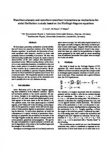
closure of the set of points where the function is not zero [32, p. 14]. For example, the support of the Heaviside function is supp H = [0, +∞[. Note that although a function is zero outside its support, it can also vanish at isolated points of its support, because of the closure condition of the definition. For example the support of the sine function is R although sin(nπ) = 0. However, the support of a distribution cannot be defined as the support of a function because the value of a distribution at a point is generally not defined. Hence we define the support by duality: we say that the point x does not belong to the support of the distribution u if and only if there is an open neighborhood U of x such that u is zero on U , in other words if hu, f i = 0 for all test functions f whose support is contained in U [36, p. 12]. For example supp δ = {0} and supp θ = [0, +∞]. Similarly, we can define the singular support of a distribution u ∈ D′ (Rn ), denoted by sing supp u, by saying that x ∈ / sing supp u if and only if there is a neighborhood U of x such that the restriction of u to U is a smooth function, in other words if R there is a smooth function φ ∈ C ∞ (U ) such that hu, f i = hφ, f i = φ(x)f (x)dx for all test functions f supported on U [36, p. 108]. For example sing supp δ = {0}, sing supp θ = {0}. A more elaborate example is the distribution u ∈ D′ (R), defined by: u(x) = (x + i0+ )−1 , i.e. u is the limit in D′ (R) of uε (x) := (x + iǫ)−1 , when ε > 0 and ε → 0, this means that [43, § 2]: Z ∞ Z ∞ f (x)dx f (x) − f (−x) hu, f i = lim = lim dx − iπf (0). x ǫ→0+ −∞ x + iǫ ǫ→0+ ǫ If y 6= 0, consider the open set U = (y − |y|/2, y + |y|/2). Take a smooth function χ such that χ(x) = 1 for |x − y| < 3|y|/4 and χ(x) = 0 for |x − y| > 7|y|/8. Then, for any f supported on U we have f (0) = 0 and f = f χ. Thus, Z ∞ χ(x)f (x) − χ(−x)f (−x) dx hu, f i = hu, χf i = x |y|/8 Z ∞ χ(x)f (x) = dx = hφ, f i, x −∞ where φ(x) = χ(x)/x is smooth because χ(x) = 0 for |x| < |y|/8 (see fig. 1). As a consequence, every y 6= 0 is not in the singular spectrum of u and sing supp u = {0} because the imaginary part of u is proportional to a Dirac δ distribution. We can now state an important theorem [32, p. 55]. Theorem 1. If u and v are two distributions in D′ (Rn ) such that sing supp u ∩ sing supp v = ∅, then the product uv is well defined. Proof. We first notice that, if f ∈ D(Rn ) is supported outside the singular support of v, then vf is smooth and we can define the product by huv, f i = hu, vf i. Similary, huv, f i = hv, uf i if f is supported outside the singular support of u. This definition of uv extends to all test functions f by using a smooth function χ which is equal to zero on a neighborhood of the singular support of u and equal to one on a neighborhood of the singular support of v. Then huv, f i = hv, uχf i + hu, v(1 − χ)f i. This product is associative and commutative [32, p. 55]. 2.1.3. The singular oscillations of the distributions are transversal Consider R the two distributions Ru = δ ⊗ 1 and v = 1 ⊗ δ in D′ (R2 ), i.e., ∀ϕ ∈ D(R2 ), hu, ϕi = R ϕ(0, y)dy and hv, ϕi = R ϕ(x, 0)dx. Then we can define their product by uv = (δ ⊗ 1)(1 ⊗ δ) :=


5

1.2

Χ 1.0

0.8

0.6

0.4

0.2

U 0.0 0.0

0.5

y 1.0

1.5

Figure 1. In this figure we take y = 0.8, the open set is U = (0.4, 1.2) and the smooth function χ is supported on (0.1, 1.5).

RR (2) u(x)v(y)ϕ(x, y)dxdy = Rδ ⊗ δ =R δ , i.e. huv, ϕi = R ϕ(0, 0), since huv, ϕi = u(x) v(y)ϕ(x, y)dy dx = u(x)ϕ(x, 0)dx = ϕ(0, 0) by the Fubini theorem for distributions. Here u and v are singular on the lines {x = 0} and {y = 0} respectively, which have a non empty intersection {(0, 0)}. However the oscillations of both distributions are orthogonal at that point, so that this definition makes sense. But actually the orthogonality is not essential and, as we will see, the important point is the transversality. Indeed we can extend this example to measures which are supported by non orthogonal lines: let α : R2 −→ R2 be a linear invertible map and set α = (α1 , α2 ) and uα := α∗ u = u ◦ α and vα := α∗ v = v ◦ α, where ∀w ∈ D′ (R2 ), ∀ϕ ∈ D(R2 ), hα∗ w, ϕi := (detα)−1 hw, ϕ ◦ α−1 i. These distributions are well-defined and they are singular on the line of equation α1 = 0 and α2 = 0 respectively. Moreover we can define uα vα by setting uα vα := α∗ (uv) = α∗ (δ (2) ). Hence here uα vα = (detα)−1 δ (2) and we see that the product makes sense as long as detα 6= 0, which means that the singular supports of uα and vα are transversal. 2.1.4. The singularities of the distributions are transversal in the complex world This last case looks as the most mysterious at first glance and concerns complex valued distributions. Consider the distribution u(x) = 1/(x + i0+ ) defined previously, i.e. iε x the limit of uǫ (x) = 1/(x + iε) = x2 +ε 2 − x2 +ε2 when ε > 0 and ε → 0. (Hence 1 u = pv( x ) − iπδ0 .) Observe that (uε )′ = −(uε )2 , ∀ε > 0. Thus since (uε )′ converges to u′ in D′ (R), we can set u2 := −u′ . Moreover since any polynomial relation in uε and its derivatives which follows from Leibniz rule is satisfied (uε being a smooth function), the same holds for u. One can define similarly the square of u(x) = 1/(x − i0+ ). However this recipe fails for defining the product of u by u. A similar mechanism works for making sense of the square of the Wightman function (see Section 6). One way to understand what’s happening is to remark that we multiply distributions which are boundary values of holomorphic functions on the same domain. In order to really understand all these examples and go beyond, we need to revisit them by using refined tools such as: the Radon transform and the Fourier transform.


6

This will lead us to H¨ ormander’s definition of wavefront sets. 2.2. The product of distributions by using Fourier transform We remark that the Fourier transform of a product of distributions (when it is defined) is the convolution of the Fourier transforms of these distributions [36, p. 102]: u cv = u ˆ ⋆ vˆ, if it exists. Therefore, we can define the product of two distributions u and v as the inverse Fourier transform of u ˆ ⋆ vˆ. However, this definition, which requires the Fourier transforms of u and v to be defined and their convolution product to make sense, can be improved. Indeed it does not take into account the fact that the product of two distributions is local, i.e. that its definition on the neighbhorhood of a point depends only on the restriction of the distributions on that neighborhood. Therefore, we can localize the distributions by multiplying them with a test function: if u ∈ D′ (U ) and f ∈ D(U ), then f u is a distribution with compact support in U and we can extend it to a distribution defined on Rn by setting it to equal to zero outside U . Let us still denote by f u this compactly supported distribution on Rn . It has a Fourier transform fcu(k) which is an entire analytic function of k by the Paley–Wiener–Schwartz Theorem. Following the physicist’s convention [44],[45, p. 32], we define the Fourier transform of u by Z F (u)(k) = u ˆ(k) = dxeik·x u(x), P

Rn

i

where k · x = i ki x (we could interpret this quantity as an Euclidean scalar product between two vectors in Rn ; however as we will see in Section 6 it is better to understand k as a covector and the product k·x as a duality product, this is the reason for the lower indices used for the coordinates of k and the upper indices used for the coordinates of x). More rigorously, the above definition applies to functions f of rapid decrease and, for a tempered distribution u, the Fourier transform is defined by hˆ u, f i = hu, fî. The inverse Fourier transform is Z dk −ik·x e u ˆ(k), u(x) = (2π)n where n is the dimension of spacetime. The same convention was used, for example, by Franco and Acebal [46]. Note the relation between this Fourier transform and the one used in other references: uˆ(k) = FH (u)(−k) [32, 47], or u ˆ(k) = (2π)n/2 FRS (u)(−k) [35, 39, 41]. We can now give a definition of the product of two distributions. Note that there are alternative definitions, under different hypotheses (and we will meet another one later on). For a general overwiew about the existing options, see [48, 49]. Definition 2. Let u and v in D′ (Rn ). We say that w ∈ D′ (Rn ) is the product of u and v if and only if, for each x ∈ Rn , there exists some f ∈ D(Rn ), with f = 1 near x, so that for each k ∈ Rn the integral Z 1 d 2 c c f w(k) = (f u ⋆ f v)(k) = fcu(q)fcv(k − q)dq, (1) (2π)n

is absolutely convergent.

When it exists, this product has many desirable properties: it is unique, commutative, associative (when all intermediate products are defined) and it coincides


7

with the product of Theorem 1 when the singular supports of u and v are disjoint [35, p. 90]. Let us consider some examples. Example 3. If u = v = δ, the product is not defined. Proof. For any test function f satisfying the hypothesis of the definition, f δ(x) = R R f (0)δ(x) = δ(x) and fcδ(k) = 1, so that fcδ(q)fcδ(k − q)dq = dq, which is not absolutely convergent. Example 4. If u = v = θ, the product is well defined. R∞ Proof. For any f ∈ D(R), fcθ(k) = 0 eikx f (x)dx satisfies the uniform bounded R |fcθ(k)| ≤ kf kL1 := R |f (x)|dx. Moreover an integration by part gives us also R∞ fcθ(k) = ki [f (0) + g(k)] with g(k) := 0 eikx f ′ (x)dx and we thus have the uniform 1 (|f (0)| + kf ′ kL1 ). Hence, for any k ∈ R, |fcθ(k)| 6 C(1 + |k|)−1 bound |fcθ(k)| ≤ |k| for C = kf ′ kL1 + kf kL1 + |f (0)| and the integral defining (fcu ⋆ fcv)(k) is absolutely convergent because Z Z Z C 2 dq dq c c ˜ , ≤C f θ(q)f θ(k − q) dq ≤ (|k − q| + 1)(|q| + 1) (|q| + 1)2 R R R

where C˜ = C 2 supq

(|q|+1) (|k−q|+1)

is finite.

Example 5. If u(x) = v(x) = 1/(x + i0+ ), the product exists. Proof. By contour integration, uˆ(k) = −2iπθ(−k). Thus, Z Z ∞ 1 dq fˆ(q)ˆ u(k − q) = −i fcu(k) = fˆ(q)dq, 2π R k

tends to −2πif (0) = −2πi for k → −∞. To show that the integral in eq. (1) is absolutely convergent, we define the R +∞ smooth function F (k) = k fˆ(q)dq. The Fourier transform of a test function f is fast decreasing: for any integer N , there is a constant CN for which |fˆ(q)| ≤ CN (1 + |q|)−N [32, p. 252]. Thus, for k ≥ 0 Z ∞ CN |F (k)| ≤ CN (1 + q)−N dq = (1 + k)1−N , N −1 k is fast decreasing and for any k ∈ R Z ∞ 2CN |F (k)| ≤ CN (1 + |q|)−N dq = . N −1 −∞

Rk R 0 R +∞ Therefore, the right hand side of eq. (1) can be written −(2π)−1 ( −∞ + k + 0 )F (q)F (k− 2 q)dq. The first integral is absolutely convergent because |F (q)F (k − q)| ≤ 2CN (N − −2 1−N 1) (1 + |k − q|) , the second because the integrand is smooth and the domain is 2 finite and the third integral because |F (q)F (k − q)| ≤ 2CN (N − 1)−2 (1 + q)1−N . 2 To compute the product w = u we take f = 1 and we calculate directly Z Z c2 (k) = 1 u u ˆ(q)ˆ u(k − q)dq = −2π θ(−q)θ(q − k) = 2πkθ(−k). 2π R R


8

Note that the Fourier transform of the derivative of a distribution v is given by c2 = −ub′ i.e. u(x)2 = (x + i0+ )−2 = vb′ (k) = −ikˆ v(k). Thus we recover the relation u d + −1 − dx (x + i0 ) . Example 6. If u(x) = 1/(x + i0+) and v(x) = 1/(x − i0+), the product does not exist. Proof. We have u ˆ(k) = −2iπθ(−k) and vˆ(k) = 2iπθ(k). Thus, Z Z k 1 fcv(k) = dq fˆ(q)ˆ v (k − q) = i fˆ(q)dq, 2π −∞

which decreases fast for k → −∞ and tends to 2πif (0) = 2πi for k → +∞. We define Rk R +∞ G(k) = −∞ fˆ(q)dq and recall that F (k) = k fb(q)dq so that F + G = 2π. The right hand side of eq. (1) can be written as the limit for M → ∞ of (2π)−1 IM (k) with Z ∞ F (q)G(k − q)dq IM (k) = −M Z ∞ Z ∞ F (q)F (k − q)dq. F (q)dq − = 2π −M

−M

We saw in the previous example that the second term is absolutely convergent and for the first term we use F = 2π − G to write Z ∞ Z ∞ Z 0 Z 0 F (q)dq = F (q)dq + 2π dq − G(q)dq. −M

0

−M

−M

The decay properties of F and G imply that the first and third terms are absolutely convergent, but the second term is 2πM which diverges for M → ∞. Thus, there is no test function f with f (0) = 1 such that IM (k) converges: the product of distributions does not exist. In example 5, the distribution u2 was calculated without using the localizing test function f . In general this is not possible. For example, consider Example 7. 1 1 + , u(x) = + x + i0 x + a − i0+ with a 6= 0. Then, u2 exists. Indeed, denote by u1 and u2 the two terms on the right hand side. We showed that u21 exists and the same reasoning implies that u22 exists. The cross term u1 u2 exists because the singular support of u1 , which is {0}, is disjoint from the singular support of u2 , which is {−a}. Thus, u2 exists although the Fourier transform of u (i.e. uˆ(k) = −2iπθ(−k) + 2iπe−ika θ(k)) is slowly decreasing in both directions. Therefore, the role of the localizing test function f is not only to make the Fourier transform of f u exist (even when the Fourier transform of u does not), but also to isolate the singularities of u. In example 7, the two singular points of u are x = 0 and x = −a. To localize the distribution around x = 0, we multiply u by a smooth function f such R∞ c that f (0) = 1 and f (x) = 0 for |x| > |a|/2, so that f u(k) = −i k fˆ(q)dq is fast decreasing in the direction of k > 0 because the contribution of 1/(x + a − i0+ ) is eliminated. Conversely, if we multiply the distribution by a smooth function g such Rk that g(−a) = 1 and g(x) = 0 for |x + a| > |a|/2, then gc u(k) = i −∞ gˆ(q)dq, which is fast decreasing in the direction k < 0.


9

2.2.1. Discussion In the previous examples, we saw that the calculation of the product of two distributions by using the Fourier transform looks rather tricky. In particular, it seems that we have to know the Fourier transform of the product of each distribution with an arbitrary function. Moreover even when we are able to define it, the product of distribution does not always satisfy the Leibniz rule ∂(uv) = (∂u)v + u(∂v). For instance the product of θ makes sense (Example 4) but does not respect the Leibniz rule (see Section 2). On the other hand the square of 1/(x + i0+ ) can be defined (see Example 5) and this definition agrees with Leibniz rule. Fortunately, H¨ ormander devised a powerful condition on a pair of distributions to: 1) guarantee the existence of their product without computing it; 2) ensure that this product satisfies the Leibniz rule. As a preparation for this condition, we can analyze why the product exists in example 5 and not in example 6. In example 5, the support of uˆ is (−∞, 0) and, because of the convolution formula uˆ(q)ˆ u(k − q), the support of uˆ(q)ˆ u(k − q) as a function of q is the finite interval [k, 0] if k ≤ 0 and is empty if k > 0. Thus, the integral over q is absolutely convergent. On the other hand, in example 6 the support of u ˆ(q)ˆ v (k − q) is (−∞, min(k, 0)), which is infinite. In general, for the convolution integral to be well defined, we just need that the product fcu(q)fcv(k − q) decreases fast enough for large q for the integral over q to be absolutely convergent. Note also that, for any distribution u and for any smooth function f with compact support, since f u is a distribution with compact support, its Fourier transform fcu grows at most polynomially at infinity, i.e. there exists some p ∈ N and some constant C > 0 such that |fcu(k)| ≤ C(1 + |k|)p everywhere. Hence it is enough that one of the two factors in the product fcu(q)fcv(k − q) is fast decreasing at infinity to ensure that the product is fast decreasing. In example 5, fcu(q) decreases very fast for q → +∞ but does not decrease for q → −∞. If fcu(q) decreases slowly in some directions q, this must be compensated by a fast decrease of fcv(k − q) in the same direction q. This is exactly what happens in example 5 and not in example 6. Lastly Example 7 confirms that a general condition for the existence of a product of distributions should use the Fourier transform of distributions localized around singular points. It is now time to introduce the key notion for defining H¨ ormander’s product of distributions: the wavefront set. 3. The wavefront set We want to find a sufficient condition by which the product of distributions defined in eq. (1) is absolutely convergent. In this integral, the distribution f v is compactly supported because f ∈ D(Rn ). Thus, there is constant C and an integer m such that |fcv(k − q)| ≤ C(1 + |k − q|)m . The smallest m for which this inequality is satisfied is called the order of the distribution f v. The integral (1) would be absolutely convergent if we had |fcu(q)| ≤ C ′ (1 + |q|)−m−n−1 . However, since we also wish the product of distributions to be compatible with derivatives through the Leibniz rule ∂(uv) = (∂u)v + u(∂v) and since a derivative of order n increases the order of u by n, what we really need is that |fcu(q)| decreases faster than any inverse power of 1 + |q|. We give now a precise definition of the property of fast decrease.


10

V k0

Figure 2. Example of a conical neighborhood of k.

3.1. Outside the wavefront set: the regular directed points We start by defining some basic tools: the conical neighborhoods and the fast decreasing functions. Definition 8. A conical neighborhood of a point k ∈ Rn \ {0} is a set V ⊂ Rn such that V contains the ball B(k, ǫ) = {q ∈ Rn ; |q − k| < ǫ} for some ǫ > 0 and, for any p in V and any α > 0, αp belongs to V . An example of conical neighborhood of k is given in figure 2. Definition 9. A smooth function g is said to be fast decreasing on a conical neighborhood V if, for any integer N , there is a constant CN such that |g(q)| ≤ CN (1 + |q|)−N for all q ∈ V . 2

For example, the function e−q is fast decreasing on Rn . We need functions to be fast decreasing in a conical neighborhood and not only along a specific direction (which would be the case if CN were a function of q), because a single direction has zero measure and we would not be able to control the integral (1). According to the discussion of the previous section we see that the integral (1) converges absolutely if the directions where fcv(k − q) decrease slowly correspond to regions where fcu(q) is fast decreasing. We define now the “nice points” around which fcu is fast decreasing. They are called regular directed points [35, p. 92]: Definition 10. For a distribution u ∈ D′ (Rn ), a point (x, k) ∈ Rn × (Rn \{0}) is called a regular directed point of u if and only if there exist: (i) a function f ∈ D(Rn ) with f (x) = 1 and (ii) a closed conical neighborhood V ⊂ Rn of k, such that fcu is fast decreasing on V .

The relevance of the concept of regular directed point also stems from the following theorem [32, p. 252] Theorem 11. A compactly supported distribution u ∈ E ′ (U ) is a smooth function if and only if u b(q) is fast decreasing on Rn .


11

This theorem is physically reasonable because, if f is a smooth function, then f (x)eik·x oscillates widely when k is large, so that the average of this expression (i.e. fb(k)) is very small. Theorem 11 implies that any singularity of a distribution can be detected by an absence of fast decrease in some direction: a point x is in the singular support if and only if there is a direction k where the Fourier transform is not fast decreasing. However, if x ∈ sing supp u, there can be directions k such that (x, k) is regular directed. In example 5, we saw that fcu(k) is rapidly decreasing for k > 0 but not for k < 0. This brings us finally to the definition of the wavefront set 3.2. The definition of the wavefront set and the Product Theorem Definition 12. The wavefront set of a distribution u ∈ D′ (Rn ) is the set, denoted by WF(u), of points (x, k) ∈ Rn × (Rn \{0}) which are not regular directed for u. In other words, for each point of the singular support of u, the wavefront set of u is composed of the directions where the Fourier transform of f u is not fast decreasing, for f a sufficiently small support. The name “wavefront set” comes from the fact that the singularities of the solutions of the wave equation move within it [32, p. 274], so that the wavefront set describes the evolution of the wavefront. The wavefront set is a refinement of the singular support, in the sense that the singular support of u is the set of points x ∈ Rn , such that (x, k) ∈ WF(u) for some nonzero k ∈ Rn . Now we see how this definition can be used to determine the product of two distributions u and v. Broadly speaking, if a point x belongs to the singular support of u and v, then the product of u and v exists at x if, for all directions q, either fcu(q) or fcv(k − q) is rapidly decreasing. In particular, if (x, q) belongs to WF(u), then (x, −q) must not belong to WF(v). This is called H¨ ormander’s condition and the precise theorem is [32, p. 267]: Theorem 13 (Product Theorem). Let u and v be distributions in D′ (U ). Assume that there is no point (x, k) in WF(u) such that (x, −k) belongs to WF(v), then the product uv can be defined. Moreover, if so, then WF(uv) ⊂ S+ ∪ Su ∪ Sv ,

(2)

where S+ = {(x, k + q)|(x; k) ∈ WF(u) and (x; q) ∈ WF(v)}, Su = {(x; k)|(x; k) ∈ WF(u) and x ∈ supp (v)} and Sv = {(x; k)|(x; k) ∈ WF(v) and x ∈ supp (u)}. Remarks (i) This theorem is absolutely fundamental for the theory of renormalization in curved spacetimes. With this simple criterion, we can prove that a product of distributions exists even if we cannot calculate their Fourier transforms and even if we do not know the explicit form of the distributions. (ii) The condition involving the support of u in Sv and the support of v in Su in WF(uv) is given in [38, p. 84] but is usually not stated explicitly [32, p. 267] [33, p. 21] [35, p. 95], [34, p. 527], [36, p. 153], [37, p. 193], [40, p. 61]. This support condition is imperative to calculate the wavefront set of example 19 or of the Feynman propagator in section 6.2. (iii) When H¨ ormander’s condition holds, then the product of distributions satisfies the Leibniz rule for derivatives, because derivatives do not extend the wavefront set [32, p. 256]).


12

(iv) Note that if u and v satisfy H¨ ormander’s condition, then their product exists in the sense of Definition 2. The converse is not true in general. However, if the product of distributions is extended beyond H¨ ormander’s condition, then it is generally not compatible with the Leibniz rule, as shown by the example of the Heaviside distribution at the beginning of section 2. (v) H¨ ormander’s condition of the Product Theorem can be rephrased by saying that S+ does not meet the zero section (of the cotangent bundle over U ), i.e. that S+ ∩ (U × {0}) = ∅. (vi) For any pair A and B of subsets of U × Rn , we can define A ⊕ B := {(x, k + q)|(x, k) ∈ A, (x, q) ∈ B}. We then observe that S+ = W F (u)⊕W F (v) and hence H¨ ormander’s condition amounts to saying that W F (u)⊕W F (v) does not intersect the zero section. On the other hand if we set W F (u) := W F (u) ∪ (supp u × {0}), etc., we then always have W F (u) ⊕ W F (v) = S+ ∪ Su ∪ Sv ∪ (supp (uv) × {0}). Moreover if H¨ ormander’s condition holds then supp (uv) × {0} is disjoint from S+ ∩ Su ∩ Sv and thus Conclusion (2) is equivalent to the inclusion W F (uv) ⊂ W F (u) ⊕ W F (v). 3.3. Simple examples and applications of the Product Theorem We give a few very simple examples. Example 14. The simplest example is δ(x) in D′ (Rn ), for which WF(δ) = {(0; k)|k ∈ Rn , k 6= 0}. Thus, the powers of δ cannot be defined. Proof. The singular support of δ(x) is {0} and fcδ(k) = f (0) is not fast decreasing if f (0) 6= 0. This proves that WF(δ) = {(0; k)|k ∈ Rn , k 6= 0}. To show that the product is not allowed, consider any point (0; k) of W F (δ), then (0; −k) is also a point of WF(δ) and the H¨ ormander condition is not satisfied. Example 15. The wavefront set of the Heaviside distribution θ is WF(θ) = c (k)| ≤ C/(1 + |k|) for all k. {(0; k) ; k 6= 0}. There is a constant C such that |θf

Proof. The Heaviside distribution is smooth for x < 0 and x > 0 because it is constant there. Thus, the only possible singular point is x = 0. Consider a smooth compactly supported function f such that f (0) = 1. We have for k 6= 0 Z Z ∞ (−i) ∞ ikx ′ c (k) = (e ) f (x)dx θf eikx f (x)dx = k 0 0 Z i ∞ ikx ′ if (0) + e f (x)dx, (3) = k k 0 where the prime denotes a derivative with respect to x and we integrated by parts. A further integration by part gives us Z ∞ if (0) f ′ (0) 1 c θf (k) = − 2 − 2 eikx f ′′ (x)dx. (4) k k k 0

Let L be the length of supp f and, for n = 0, 1, 2, let Mn be a constant such that c (k) − i | ≤ |f (n) (x)| ≤ Mn for all x. Using f (0) = 1, Identity (4) implies that |θf k M1 +LM2 . Hence (0, k) ∈ W F (θ), ∀k 6= 0. On the other hand (3) implies both k2 c (k)| ≤ LM0 and |θf c (k)| ≤ 1+LM1 . We hence deduce that |θf c (k)| ≤ C , for some |θf |k| 1+|k| constant C.


13

The wavefront set of θ is the same as the wavefront set of δ. This explains why the powers of θ are not allowed in the sense of H¨ ormander. Example 16. u(x) = 1/(x + i0+ ), then WF(u) = {(0; k), k < 0}. Thus, u2 exists and WF(u2 ) = WF(u). Proof. The proof is obvious from example 5 (see also [35, p. 94], where one must recall that the sign is opposite because of the different convention for the Fourier transform). Example 17. v(x) = 1/(x − i0+), then WF(v) = {(0; k), k > 0}. Thus, v 2 exists and WF(v 2 ) = WF(v), but we cannot conclude that uv exists (it does not, as we saw in example 6). Example 18. We consider again example 7: 1 1 u(x) = + , x + i0+ x + a − i0+ with a 6= 0. Then, WF(u) = {(0; k), k < 0} ∪ {(−a; k), k > 0} and u2 exists, with WF(u2 ) = WF(u). ′ 2 Example 19. R (See [35, p. 97]). Let δ1R and δ2 be the distributions in D (R ) defined by hδ1 , f i = dyf (0, y) and hδ2 , f i = dxf (x, 0). Then, WF(δ1 ) = {(0, y; λ, 0)|y ∈ R, λ 6= 0} and WF(δ2 ) = {(x, 0; 0, µ)|x ∈ R, µ 6= 0}. Thus, δ1 δ2 exists and WF(δ1 δ2 ) ⊂ {(0, 0; λ, µ), λ 6= 0, µ 6= 0} ∪ {(0, 0; λ, 0), λ 6= 0} ∪ {(0, 0; 0, µ), µ 6= 0}, where we used supp (δ2 ) = {(x, 0)|x ∈ R} and supp (δ1 ) = {(0, y)|y ∈ R}. Note that the estimate of the wavefront set of δ1 δ2 would be much worse if the support of δ2 and δ1 had not been taken into account in Sδ1 and Sδ2 of the Product Theorem. In that case the inclusion is in fact an equality because WF(δ1 δ2 ) = {(0, 0; λ, µ), (λ, µ) 6= (0, 0)}.

Proof. Let y ∈ R, we want to calculate W F (δ1 ) at (0, y). Take a test function f (x1 , x2 ) which is equal to one around (0, y). Then, Z Z fd δ1 (k) = dx1 dx2 f (x1 , x2 )δ(x1 )eik1 x1 +ik2 x2 = dx2 f (0, x2 )eik2 x2 .

Take k = (k1 , k2 ) and observe the decay of fd δ1 (λk). If k2 6= 0 this is a fast decreasing function of λ because f (0, x2 ) is a smooth compactly supported function of x2 . If R k2 = 0, then we have fd δ1 (k1 , 0) = dx2 f (0, x2 ), which is independent of k1 , so that fd δ1 (λk1 , 0) is not fast decreasing. This proves that WF(δ1 ) has the given form. A similar proof yields WF(δ2 ). The rest follows from the fact that δ1 δ2 is the twodimensional delta function. 4. The wavefront set of a characteristic function Now that we know the definition of the wavefront set, we shall get the feel of it by studyingRin detail the characteristic distribution u of a region Ω of Rn , defined by hu, f i = Ω f (x)dx. We shall also revisit it in section 5.2.


14

4.1. The upper half-plane For concreteness we start from the characteristic distribution of the upper half-plane Z ∞ Z ∞ dx1 hu, f i = dx2 f (x1 , x2 ). −∞

0

This is the distribution corresponding to the function equal to one on the upper halfplane (i.e. if x2 ≥ 0) and to zero on the lower half-plane (i.e. if x2 < 0). It is intuitively clear that the singular support of u is the line (x1 , 0). Now take a point (x1 , 0) of the singular support and a test function f which is non-zero on (x1 , 0). What are the directions of slow decrease of fcu? It seems clear that fcu(k) decreases fast when k is along (1, 0), because we do not feel the step of u if we walk along it and do not cross it. But what about the other directions? Does the wavefront set contain all the directions that cross the step or just the direction (0, 1) which is perpendicular to it? The wavefront set of u can be obtained by noticing that u is the (tensor) product of the constant function 1 for the variable x1 by the Heaviside distribution θ(x2 ). Then, a standard theorem [32, p. 267] gives us WF(u) = {(x1 , 0; 0, λ), λ 6= 0}. In other words, the wavefront set detects the direction perpendicular to the step. It is instructive to make an explicit calculation to understand why it is so. We use an idea of Strichartz [37, p. 194] and consider test functions f (x1 , x2 ) = f1 (x1 )f2 (x2 ). This is not really a limitation because any test function can be c (k) = fb1 (k1 )θf c2 (k2 ). We approximated by a finite sum of such products. Then uf want to show that, if k1 6= 0, for every integer N there is a constant CN such that c (τ k)| ≤ CN (1 + τ |k|)−N for every κ > 0. We already know that there is a constant |uf DN such that |fb1 (τ k1 )| ≤ DN (1 + τ |k1 |)−N because f1 is smooth and a constant C such that |fb2 (τ k2 )| ≤ C(1 + τ |k2 |)−1 (see Example 15). We are going to show that, if the component k1 of k is not zero, the fast decrease of fb1 (τ k1 ) induces the fast c (τ k). If k1 6= 0, we have |k| ≤ α|k1 | where α = |k|/|k1 |. Note that α ≥ 1 decrease of uf because |k1 | ≤ |k|. Hence (1 + τ |k|) ≤ α(1 + τ |k1 |) and c (τ k)| ≤ CDN (1 + τ |k1 |)−N (1 + τ |k2 |)−1 ≤ CDN αN (1 + τ |k|)−N , |uf

c (τ k)| ≤ CN (1 + where we bounded (1 + τ |k2 |)−1 by 1. Finally, if k1 6= 0, then |uf τ |k|)−N for all κ > 0 with CN = αN CDN . This result was obtained for a single vector k, but it can be extended to a cone around k by increasing the value of α. 4.2. Characteristic function of general domains More generally, we can consider the characteristic function of any domain Ω in limited by a smooth surface S. The characteristic function of Ω is the function such that χΩ (x) = 1 if x ∈ Ω and χΩ (x) = 0 if x ∈ / Ω. The R characteristic function corresponds to a distribution uΩ defined by huΩ , f i = Ω f (x)dx. The wavefront of uΩ is given by [50, p. 129]:

Rn χΩ χΩ set

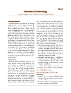
Proposition 20. Let Ω ⊂ Rn be a region with smooth boundary S and let uΩ = χΩ be the characteristic distribution of Ω. Then WF(uΩ ) = {(x, k); x ∈ S, and k normal to S}. Notice that the vectors k are perpendicular to the boundary S of Ω (see fig. 3 for the example of a disk). This can be understood by a hand-waving argument. Since the boundary S is smooth, by using a test function with very small support around


15

Figure 3. The characteristic function of the unit disk (pink) is equal to 1 for x2 +y 2 ≤ 1 to zero for x2 +y 2 > 1. Some vectors of the wavefront set are indicated as green arrows. For a given point (x, y) of the boundary x2 + y 2 = 1, the points (x, y; kx , ky ) of the wavefront set are such that (kx , ky ) is perpendicular to the boundary, thus (kx , ky ) = (λx, λy) for all λ 6= 0. In this figure we represent the characteristic function, the tangent bundle and the cotangent bundle in the same coordinates.

x ∈ S, the boundary looks flat around x and we can apply the argument of the upperhalf plane (generalized to Rn ) previously discussed. The set of vectors k which are perpendicular to all tangent vectors to S at x is called the conormal of S at x and is denoted by Cx (see fig. 3 for the example where n = 2 and Ω is the unit disk). The set C = {(x, k) ; k ∈ Cx } is called the conormal bundle of S. The previous proposition says that the wavefront set of uΩ is the conormal bundle of S. The wavefront set of a characteristic distribution has many applications. Its ability to give an accurate description of the boundary of shapes makes it particularly efficient for image analysis [51] and tomography [52]. 4.3. Counting intersections We close this section by showing that the wavefront set of the characteristic distribution of a bounded smooth domain Ω in the plane can be determined by the following striking procedure. For each straight line Lk,a in the plane, denote by nk,a the number of times the straight line intersects the boundary. For generic domains, the wavefront set of uΩ can be recovered from the set of integers nk,a [53]. In particular, this information is sufficient to recover the shape of Ω. This remark can have applications in image analysis. In some exceptional cases, this result holds only up to localization or the replacement of the number of intersections by the number of connected parts of the intersection [53]. This characterization of the wavefront set can be extended to surfaces in R3 if we replace the number of intersections nk,a by the Euler characteristic of the intersection of a given surface with all possible half–spaces [53].


16

W

4

3 2

1 0

Figure 4. Counting the number of times a straight line crosses the boundary of Ω. From the bottom to the top, this number is 0, 1, 2, 3 and 4. It is possible to reconstruct Ω from the set of straight lines and their numbers of crossings.

5. Use of the Radon transform 5.1. The wavefront set of a measure supported by a hypersurface In an attempt to better understand the wavefront set, we came up with the following idea. As seen in Example c) in Section 2.1, a distribution may be singular and may enjoy partial regularity properties simultaneously. Consider for instance a smooth submanifold Γ ⊂ Rn and the distribution which is the measure µ supported by Γ with the Euclidean density. The singular character of µ shows up by restricting µ to a smooth path which crosses transversally Γ: this gives us a Dirac mass type singularity. However if we probe µ by moving in a parallel to Γ we may be tempted to say that heuristically the distribution varies smoothly. Such a test cannot be performed by following a path which lies inside Γ, because the restriction of µ to such a path would not make sense! However we may replace such a path by a dual wave. In the most naive approach, this consists in a family of hypersurfaces (Ht )t which cross transversally (e.g. orthogonally) our path and which forms locally a foliation of an open subset of Rn . Each Ht can be thought as a wavefront in this Huygens type picture. This is another indication that we must interpret p as a covector. Let’s explore this idea in the simple case where Γ is a smooth curve. Choose a point x0 ∈ Γ and a covector p ∈ Rn , and define the linear form α : Rn −→ R by α(x) := p · x and assume that α|Tx0 Γ 6= 0. We will test µ locally around x0 by using a plane wave whose wavefronts are the hyperplanes Hα,a of equation α(x) = a, for a ∈ R close to α(x0 ). Choose an open neighborhood U ⊂ Rn of x0 such that there exists a parametrization γ : I −→ U of Γ ∩ U . Then for any ϕ ∈ D(Rn ) with support contained in U , we have Z ˙ hµ, ϕi = ϕ(γ(t))|γ(t)|dt. I


17

Moreover we may choose U such that α|Tx Γ 6= 0, ∀x ∈ Γ ∩ U . We remark then that α ◦ γ is a diffeomorphism into its image. Let ω be an open subset of U such that ω ⊂ U and let χ ∈ D(Rn ) with support contained in U and such that χ = 1 on ω. Let f ∈ D(R) with support in α(ω ∩ Γ). Set ϕ := χ(f ◦ α) and observe that f ◦ α = ϕ on U ∩ Γ. Hence we can define hµ, f ◦ αi by setting Z ˙ hµ, f ◦ αi := hµ, ϕi = f ◦ α ◦ γ(t)|γ(t)|dt. I

By performing the change of variable a = α ◦ γ(t), da = |α(γ(t))|dt, ˙ A = α ◦ γ(I), we obtain Z da f (a) , hµ, f ◦ αi = |α(τ (a))| A where τ (a) is the tangent vector to Γ: τ (α ◦ γ(t)) = γ(t)/| ˙ γ(t)|. ˙ We see that we can extend this definition by replacing f by a Dirac mass δa at some value a ∈ A. We then get hµ, α∗ δa i = 1/|α(τ (a))| = 1/|p · τ (a)|, a smooth function of a. However it appears clearly that this quantity becomes singular when α(τ (a)) = p · τ (a) = 0: this corresponds to points of Γ such that Tx Γ is contained in the kernel of α. Note that we may replace α by α e(x) = pe · x, for pe ∈ Rn close to p: by choosing U suitably we can show that the previous computation remains valid for (e α, a) close to (α, α(x0 )). Geometrically hµ, α e∗ δa i corresponds to the integral of µ on the hyperplane Hαe,a (more precisely a neighborhood in Hαe,a of x0 ), i.e. the value of the local Radon transform at this hyperplane. 5.2. The Radon transform of the characteristic function of the half-plane We go back to the distribution u introduced in Section 4.1, i.e. the characteristic function of the upper half-plane Ω in R2 . Any half-line {(x, λk)|λ ∈ (0, +∞)} in the wavefront set of u is characterized by a point x and a unit direction k. Consider a straight line perpendicular to k and move it along k. Then, something should happen to the restriction of u to the line when the line crosses the point x. To be more precise, consider a straight line Lk,a defined by the equation k ·x = a (the line perpendicular to k that goes through the point (a/k1 , 0) if k1 6= 0). By changing the valueR of a we move the line along k. The integral of f u over the line Lk,a is R(f u)(k, a) = Lk,a ∩Ω f (x)dℓ is the value of the Radon transform of f u at (k, a). Let us check in this case the result which will be proved in section 5.3, i.e. that the wavefront set of u Rcan be obtained by looking at the points where the Radon transform R(f u)(k, a) = Lk,a ∩Ω f (x)dℓ is not a smooth function of a. This means here that if a line Lk,a is not parallel to the step, then a small variation of a is smooth, while it will jump at the step if Lk,a is the x1 axis (see Fig. 5). To prove this, let k be a unit vector and v a unit vector perpendicular to k. Then the points of the straight line Lk,a are x = ak + tv and Z ∞ R(f u)(k, a) = f (ak + tv)θ(ae2 · k + te2 · v)dt, −∞

where e2 is the unit vector along the x2 axis. If we choose an angle −π/2 < φ ≤ π/2 such that k = e1 sin φ + e2 cos φ and v = e1 cos φ − e2 sin φ (where e1 is the unit vector R∞ along the x1 axis) we obtain R(f u)(k, a) = −∞ f (ak + tv)θ(a cos φ − t sin φ)dt. We


18

Figure 5. The upper half-plane is green. An integration over the blue lines (which are not parallel to the edge) gives a smooth function of the distance from the first line. An integration over the red lines (parallel to the edge) jumps when the line reaches the edge.

must consider three cases. R(f u)(k, a) =

Z

∞

f (ak + tv)dt if φ > 0,

acotgφ Z ∞

R(f u)(k, a) = θ(a) R(f u)(k, a) =

Z

f (ae2 + te1 )dt if φ = 0 and a 6= 0,

−∞ acotgφ

f (ak + tv)dt if φ < 0.

−∞

We indeed see that R(f u)(e2 , a) jumps from 0 for a = 0− to

R∞

−∞

f (te1 )dt for a = 0+ .

5.3. The wavefront set up to sign and the Radon transform Let us start with the following definition: Definition 21. For any distribution u the wavefront set up to a sign of u is the set WF± (u) := {(x, p)|(x, p) ∈ WF(u) or (x, −p) ∈ WF(u)}. This notion is slightly coarser than the wavefront set. However it gives interesting information about its geometry. Note that T ∗ M \ WF± (u) is the set of absolutely regular directed points. These are the points (x, p) such that there exists f ∈ D(Rn ) satisfying f (x) = 1 and a closed conic neighborhood V ⊂ Rn of p such that fcu is fast decreasing on V ∪ (−V ). The set WF± (u) or equivalently its complementary set can be characterized by using the Radon transform. Radon transform is defined by averaging functions on affine subspaces. Here we use affine hyperplanes of Rn . First consider the case of a continuous function with compact support u ∈ Cc0 (Rn ). For any (ν, s) ∈ S n−1 × R, let Hν,s be the hyperplane of equation ν · x = s and set Z u(x)dσ(x), R(u)(ν, s) := Hν,s

where σ is the Lebesgue measure on Hν,s . This defines a function R(u) on S n−1 × R, the Radon transform of u. This function is linked to the Fourier transform of u by Z Z ip·x ds eis|p| R(u) (p/|p|, s) dx e u(x) = u b(p) = R Rn p = F R(u) ,· (|p|), |p|

Introduction to the wavefront set hence conversely R(u)(ν, s) =

1 2π

19 Z

R

dk e−iks u b(kν).

Now consider a distribution u ∈ D′ (Rn ), let (x, p) be an absolutely regular directed point of u. Let f ∈ D(Rn ) such that f (x) = 1 and a closed conic neighborhood V ⊂ Rn of p such that fcu is fast decreasing on V . For any ν ∈ V ∩ S n−1 , k 7−→ fcu(kν) is a smooth fast decreasing function of k ∈ R. We can thus define its inverse Fourier transform and set Z 1 dk e−iks fcu(kν). R(f u)(ν, s) = 2π R

Note, for any fixed ν, s 7−→ R(f u)(ν, s) has a compact support because f has a N compact support. Since ∀N ∈ N, ∃Cn > 0 such that ∀q ∈ V , |fcu(q)| ≤ CN (1 + |q|) , m d ′ it implies that, ∀m ≤ N − 2, ∀ν ∈ V ∩ S n−1 , (ds) m R(f u)(ν, s) ≤ C CN , for R dk 1 . Hence R(f u) is uniformly smooth in s on (V ∩ S n−1 ) × R. C ′ = 2π R (1+|k|)2 Conversely let u be a distribution and assume that, for some (x, ν) ∈ Rn × S n−1 , there exists f ∈ D(Rn ) and a closed neighborhood V ∩ S n−1 of ν in S n−1 such that we can make sense of the Radon transform R(f u) of f u on (V ∩ S n−1 ) × R (e.g. by proving that there exists a sequence (f u)ε of smooth functions with compact support which converges to f u in D′ (Rn ) and that the sequence R((f u)ε ) converges also in D′ (S n−1 × R) to a distribution which we call R(f u)). Conversely let u be a distribution and observe that, for any f ∈ D(Rn ) and any closed neighborhood V ∩ S n−1 of ν in S n−1 , we can make sense of the Radon transform R(f u) of f u on (V ∩ S n−1 ) × R, e.g. by noticing that f u is a compactly supported distribution, thus fcu is real analytic with polynomial growth by Paley–Wiener–Schwartz, therefore the restriction fcu(kν) is analytic with polynomial growth in k ∈ R uniformly in ν ∈ V ∩ Sn−1 , hence a tempered distribution in S ′ (R). Its inverse Fourier transform R(f u)(ν, s) is thus a tempered distribution in s.). Assume moreover, dm ∀N ∈ N, ∃ΓN > 0 such that ∀η ∈ V , (ds)m R(f u)(ν, s) ≤ ΓN . Then, since ∀η ∈ V ∩ S n−1 , s 7−→ R(f u)(η, s) is compactly supported we can define its Fourier R transform in s and set fcu(p) = R ds ei|p|s R(f u)(p/|p|, s), ∀p ∈ V . It follows then that |fcu(p)| ≤ ΓN |suppR(f u)(p/|p|, ·)||p|−N and hence fcu is fast decreasing in V . As a conclusion: Theorem 22. Let u ∈ D′ (U ) be a distribution and (x, k) ∈ U × (Rn \ {0}). Then (x, k) does not belong to W F ± (u) iff there exists f ∈ D(U ) such that R(f u) is smooth on a neigborhood of (k/|k|, k · x/|k|) in U × (V ∩ S n−1 ). 6. Oscillatory integrals In proposition 20, the singular support of the characteristic distribution is the submanifold S. H¨ ormander gives another example of a distribution where the singular support is a submanifold [32, p. 261]. This example is important because it exhibits a distribution defined by an oscillatory integral (as the Wightman propagator). Example 23. Let M be a smooth submanifold of Rn defined near a point x0 ∈ M by φ1 (x) = . . . = φk (x) = 0 where dφ1 , . . . , dφk are linearly independent at x0 . If the function a ∈ D(Rn ) has support near x0 , we define the distribution hu, f i =

Introduction to the wavefront set 20 R (2π)k dxa(x)δ(φ1 , . . . , φk )f (x), where δ is the delta function in Rk . This can be rewritten Z Z hu, f i = dxf (x) dξ a(x)eiφ(x,ξ) , Pk

Rn

Rk

where φ(x, ξ) = i=1 φi (x)ξi and ξi ∈ R. Then W F (u) = {(x, −dx φ(x, ξ)); φ1 (x) = . . . = φk (x) = 0, x ∈ supp a}, where ∂φ(x, ξ) ∂φ(x, ξ) dx1 + . . . + dxn . ∂x1 ∂xn We can use this result to recover the wavefront set of example 20 when n = 2, Ω is the unit disk and S is the unit circle. We have a single function φ1 (x1 , x2 ) = x21 +x22 −1, so that φ(x, ξ) = (x21 + x22 − 1)ξ, the critical set is given by dξ φ(x, ξ) = φ1 (x1 , x2 ) = 0 and dx φ(x, ξ) = (2x1 dx1 + 2x2 dx2 )ξ. If we switch to polar coordinates, we obtain dx φ(x, ξ) = 2ρξdρ, which is a direction perpendicular to the unit circle at x. Note that ξ can have both signs, thus both dρ and −dρ belong to the wavefront set. This example confirms an important characteristics of the wavefront set. The direction k are not vectors but covectors. Indeed, dx φ(x, ξ) can be expanded over the (covector) basis dx1 , . . . , dxn of Tx∗ M and not over the vector basis ∂x1 , . . . , ∂xn of Tx M . To determine the nature of the directions k in the wavefront set, we can also look at the way the wavefront set transforms under a smooth mapping Rn → Rn . The detailed calculation [37, p. 195] confirms that k are covectors because they transform covariantly. This point is important for distributions on manifolds. The previous result can be extended to more generaly oscillatory integrals (in the following we always assume that the phase function φ is homogeneous of degree 1, i.e. φ(x, λξ) = λφ(x, ξ), ∀λ > 0, see [32, p. 260] for details): dx φ(x, ξ) =

Theorem 24. If a distribution u is defined by an oscillatory integral Z Z dξ a(x, ξ)eiφ(x,ξ) dξ, dxf (x) u(f ) = Rn

Rs

where φ is a phase function and a an asymptotic symbol, then W F (u) ⊂ {(x; −dx φ(x, ξ)) | dξ φ(x, ξ) = 0}. We refer to the literature for a precise definition of phase functions and asymptotic symbols [32, p. 236][35, p. 99]. We can give a hand-waving argument to the origin of this wavefront set. The Fourier transform of u is given by R understand R dx dξa(x, ξ)eiφ(x,ξ)+ik·x . By using the stationary-phase method, we see that the directions of slow decrease are the directions where the phase φ(x, ξ) + k · x is critical with respect to (x, ξ). They are determined by the equations k + dx φ(x, ξ) = 0 and dξ φ(x, ξ) = 0. 6.1. The Wightman propagator With the help of theorem 24 we can calculate the wavefront set of a fundamental distribution of quantum field theory: the Wightman propagator in Minkowski spacetime [35, p. 66] Z dxdyh0|ϕ(x)ϕ(y)|0if (x)g(y) W2 (f, g) = R3 ×R3 Z dxdy∆+ (x − y)f (x)g(y), = −i R3 ×R3


21

Figure 6. Wavefront set of ∆+ : the wavefront set at the origin is an upper cone. Note that, in this figure, three different spaces are identified: the configuration space R3 , the tangent space and the cotangent space over each point of the configuration point. The tangent and cotangent spaces are identified through the Euclidian metric. This implies that the covectors in WF(u) are perpendicular to the tangent planes.

where [35, p. 70]

Z dk −ik·x i e , 2(2π)3 R3 k0 p P3 with k = (k1 , k2 , k3 ), k0 = |k|2 + m2 , k = (kµ ) = (k0 , k) and k · x = µ=0 kµ xµ . The analytic form of ∆+ (x) is given by Scharf [54, p. 90]. We can write ∆+ (f ) in the oscillatory integral form of Theorem 24 by setting, for ξ ∈ R3 , [35, p. 100] ∆+ (x) =

0

j

φ(x, ξ) = − x |ξ| − x ξj ,

a(x, ξ) =

e−ix

0

(ωξ −|ξ|)

ωξ

,

p p P where |ξ| = (ξ1 )2 + (ξ2 )2 + (ξ3 )2 , ωξ = |ξ|2 + m2 and xj ξj = 3j=1 xj ξj . To prove this, just write −ik · x = − i(xj kj + x0 k0 ) = i(−x0 |k| − xj kj ) − ix0 (k0 − |k|), and replace k by ξ. The modification of the phase is necessary to make a(x, ξ) an asymptotic symbol. We can now calculate the wavefront set of the Wightman propagator [35, p. 106] Proposition 25. The wavefront set of ∆+ is WF(∆+ ) = S0 ∪ S+ ∪ S− , where S0 = {(0; |k|, k) | k ∈ (R3 \{0})}, S± = {(±|x|, x; λ|x|, ∓λx) | x ∈ (R3 \{0}), λ > 0}. More compactly [39, p. 118], WF(∆+ ) = {(x; k) ; k0 = |k|, x0 = λk0 , xi = −λki , λ ∈ R}. The advantage of the physical convention for the Fourier transform is that positive energies correspond to k0 > 0. The wavefront set of ∆+ for curved (globally hyperbolic) spacetime is given by Strohmaier [39]. Proof. According to Theorem 24, we first calculate the set of critical points {dξ φ = 0} P3 ξi dξi P3 0 i 0 for φ(x, ξ) = −x |ξ|− x ξi . We find −x − i=1 xi dξi = 0, which implies i=1 |ξ|


22

Figure 7. Wavefront set of ∆F , the wavefront set at the origin is a ball.

ξi xi = −x0 |ξ| and thus x0 = λ|ξ| and xi = −λξi for λ =

x0 |ξ| .

Conversely, if we plug P3 x = λ|ξ|, x = −λξi in dξ φ for any λ ∈ R, we find dξ φ = i=1 (λξi − λξi )dξi = 0. Then Theorem 24 claims that W F (∆+ ) is a subset of {(x; dx φ) ; dξ φ(x; ξ) = 0}: 0

i

W F (∆+ ) ⊂ {(x0 , x; |ξ|, ξi )|x0 = λ|ξ|, xi = −λξi , λ ∈ R} ⊂ {(x0 , x; k0 , ki )|k0 = |k|, x0 = λk0 , xi = −λki , λ ∈ R}. We leave to the reader the proof of the decomposition {(x0 , x; k0 , ki )|k0 = |k|, x0 = λk0 , xi = −λki , λ ∈ R} = S0 ∪ S+ ∪ S− . Note that theorem 24 states only that WF(∆+ ) ⊂ S0 ∪ S+ ∪ S− . We refer to the literature to show that ⊂ can be replaced by = [35, p. 107]. The singular support of ∆+ is the light cone x0 = ±|x|, the cotangent vectors k are light-like, have positive energy k0 and are perpendicular to x. 6.2. The Feynman propagator Proposition 26. The Feynman propagator ∆F (x) = θ(x0 )∆+ (x) + θ(−x0 )∆+ (−x) exists and its wavefront set is WF(∆F ) = D∗ ∪ CF , where D∗ = {(0; k) | k 6= 0} is the wavefront set of the Dirac delta function and CF = {(x; k) | (x0 )2 − |x|2 = 0, x0 6= 0, k0 = λx0 , ki = −λxi , λ > 0}. Proof. θ(x0 )∆+ (x) is a product of distributions, we must Rfirst show that it exists. As a distribution in R4 , θ(x0 ) is defined by θ(x0 )(f ) = x0 >0 f (x)dx. Therefore, it is the tensor product of the Heaviside distribution in the variable x0 by the unit distribution in the variables x1 , . . . , x3 : θ(x0 ) = θ ⊗ 1. The distribution 1 is smooth and its wavefront set is empty. Thus, by property (i) of section 7, we have WF(θ(x0 )) ⊂ {(0, x; ±λ, 0) | x ∈ R3 , λ > 0}. In fact, the inclusion can be replaced by an equal sign [35, p. 108]. By theorem 13, we see that the product θ(x0 )∆+ (x) exists. Indeed, sing supp θ(x0 ) ∩ sing supp ∆+ = {0} and, at x = 0, the allowed cotangent vectors are k = (±λ, 0) with λ > 0 for θ(x0 ) and q = (|k|, k) with k 6= 0 for ∆+ . Thus, q+k 6= 0 and the product exists. A similar calculation for θ(−x0 )∆F (−x) shows that ∆F is a well defined distribution on R4 . However, the estimate of the wavefront set given by the Product Theorem is not precise enough because of the contribution of WF(θ). To calculate the wavefront set of ∆F , we use the causality method of


23

Bogoliubov. Let x = (x0 , x) ∈ R4 \ {0}. If x0 > 0 then there is a neighborhood U of x such that ∀y ∈ U, y 0 > 0. Therefore, ∆F |U = θ(x0 )∆+ (x)|U = ∆+ (x)|U thus W F (∆F |U ) = W F (∆+ |U ) = S+ |U and by definition of S+ : W F (∆F |U ) = {(x; k) ; x0 = |x|, x0 = λk0 , xi = −λki , λ > 0, x ∈ U }. If x0 < 0 then there is a neighborhood U of x such that ∆F |U = θ(−x0 )∆+ (−x)|U = ∆+ (−x)|U . Thus W F (∆F |U ) = {(x; k) ; (−x; −k) ∈ S+ , x ∈ U } = {(x; k) ; x0 = −|x|, x0 = λk0 , xi = −λki , λ > 0, x ∈ U }. If x0 = 0, then x is space-like because x 6= 0. Thus, there exists some orthochronous Lorentz transformation R ∈ SO↑ (1, 3) such that (Rx)0 > 0. From the definition of ∆F we deduce that ∆F (Rx) = θ((Rx)0 )∆+ (Rx) + θ(−(Rx)0 )∆+ (−Rx). Since ∆F and ∆+ are invariant by orthochronous Lorentz transformations, this implies ∆F (x) = θ((Rx)0 )∆+ (x) + θ(−(Rx)0 )∆+ (−x). Hence we recover the case x0 > 0 and ∆F is smooth on a neighborhood of x because x is not light-like. This gives us WF(∆F )|x6=0 = CF . To complete the proof of the proposition, recall that ( + m2 )∆F = −iδ [44, p. 124]. Thus property (h) of section 7 implies WF(δ) = D∗ ⊂ WF(∆F ). Since no wavefront set at x = 0 can be larger than D∗ , we obtain WF(∆F )|x=0 = D∗ and the proposition is proved. The calculation of WF(∆F ) was first made by Duistermaat and H¨ ormander [55] after discussion with Wightman. The analytic expression for the Feynman propagator in position space is given by Zhang et al. [56]. The wavefront set of the advanced and retarded solutions to the wave equation is calculated in [55] and [39, p. 115]. 7. Properties of the wavefront set We now give without proof a number of properties of the wavefront set. Let u and v ∈ D′ (Rn ). Then (a) WF(u) is a closed subset of Rn × (Rn \{0}) [35, p. 92]. (b) For each x ∈ Rn , WFx (u) = {k ; (x, k) ∈ WF(u)} is a cone, i.e. k ∈ WFx (u) and λ > 0 implies λk ∈ WFx (u) [35, p. 92]. (c) WF(u + v) ⊂ WF(u) ∪ WF(v) [35, p. 92]. (d) sing supp u = {x ; W Fx (u) 6= ∅} [35, p. 93]. (e) If u is a tempered distribution and uˆ has support in a closed cone C, then for each x, WFx (u) ⊂ C [35, p. 93]. (f) Let U ⊂ Rm and V ⊂ Rn be two open sets. f : U −→ V we define

For any smooth (C ∞ ) map

Nf := {(f (x), k) ∈ V × Rn ; k ◦ dfx = 0}, where k ◦ dfx := (ki dy i ) ◦ dfx := ki dfxi . Consider the pull-back operator u 7−→ f ∗ u := u ◦ f defined on smooth maps u on V . Then it is possible to extend this operator to the space of distributions u ∈ D′ (V ) which satisfy Nf ∩ W F (u) = ∅ in an unique way (if we furthermore require some continuity


24

assumptions, see [32, Thm 8.2.4]). Moreover the wavefront set of f ∗ u is contained in the set f ∗ W F (u) := {(x, k ◦ dfx )|(f (x), k) ∈ W F (u)}.

(g) (h) (i) (j)

[32, Thm 8.2.4] (beware that, in the definition of the inverse image of a distribution by a diffeomorphism in [35, p. 93], the expression for the wavefront set of f ∗ u is not correct.) If u ∈ D′ (U ) and f ∈ C ∞ (U ), then WF(f u) ⊂ {supp f × (Rn \{0})} ∩ WF(u) [41, p. 344]. If u ∈ D′ (U ) and P is a partial differential operator with smooth coefficients, then WF(P u) ⊂ WF(u) [32, p. 256]. ′ If u ∈ D′ (U ) and v ∈ D (V ), then WF(u ⊗v) ⊂ WF(u) × WF(v) ∪ (supp u × {0}) × WF(v) ∪ WF(u) × (supp v × {0}) [32, p. 267]. If u ∈ D′ (U × U ) is such that (formally) u(x, y) = v(x − y) for some v ∈ D′ (V ), then WF(u) = {(x, y; k, −k) ; (x − y; k) ∈ WF(v)} [39, p. 118] and [32, p. 270].

As an application of the pull-back theorem, we calculate the wavefront set of ∆F for a massless particle, whose analytic expression is [44, p. 133] 1 1 , ∆F (x) = 2 2 4π x − i0 where x2 = (x0 )2 −|x|2 . We first prove that this distribution is well defined on R4 \{0}. −1 So ∆F is just the pull–back of (2π)−2 (t − i0) by the C ∞ map. f : x ∈ R4 \ {0} 7−→ (x0 )2 − |x|2 ∈ R.

(5) 0

0

i

i

Indeed, this map is smooth and Nf = {(f (x), k) ; 2k(x dx − x dx ) = 0}. We know that WF(1/(t − i0+ )) = {(0; k) ; k > 0}. Thus, the condition Nf ∩ W F (u) = ∅ implies x 6= 0 and ∆F is therefore well defined in D′ (R4 \ {0}). Furthermore, by property (f) W F (∆F |x6=0 ) is included in the pull–back of WF(1/(t − i0+ )) by f . We obtain: −1

W F (∆F |x6=0 ) ⊂ {(x; λ ◦ df ) ; (f (x); λ) ∈ W F (t − i0)

}.

0

Therefore, W F (∆F |x6=0 ) = {(x; k)|f (x) = 0, k = λdf (x) ⊂ λ(x , −x), λ > 0, x 6= 0}. To conclude, observe that ∆F is a homogeneous distribution, therefore by a theorem of H¨ ormander ([32, Thm 3.2.4]), it admits an extension in D′ (R4 ). The wavefront set of ∆F at x = 0 is calculated as in the proof of Prop. 26 by using ∆F = −iδ and we recover Prop. 26 for m = 0. 8. The many faces of the wavefront set In this section we give several definitions of the wavefront set. Each of them can be useful in specific contexts. 8.1. The frequency set It is possible to define the wavefront set in terms of the frequency set of distributions u, denoted by Σ(u) [32, p. 254], which is the projection of the wavefront set of u on the momentum (i.e. cotangent) space: Definition 27. Let u ∈ E ′ (Rn ), we define Σ(u) to be the closed cone in Rn \{0} having no conic neighborhood V such that, |ˆ u(k)| ≤ CN (1 + |k|)−N for k ∈ V and for all N = 1, 2, . . ..


25

Friedlander and Joshi define the frequency set Σ(u) by Definition 28. Let u ∈ E ′ (Rn ), then the direction k0 is not in Σ(u) ⊂ Rn \{0} iff ′ there is a conic neighborhood V of k0 such that, for all N , there is a CN such that ′ −N 2 1/2 |ˆ u(k)| ≤ CN hki , for all k in V , where hki = (1 + |k| ) . Duistermaat (implicitly) proposed a third definition Definition 29. Let u ∈ E ′ (Rn ), then the direction k0 is not in Σ(u) ⊂ Rn \{0} iff there is a neighborhood W of k0 such that, for all N , there is a constant DN such that |ˆ u(τ k)| ≤ DN τ −N for τ → ∞ uniformly in k ∈ W . The proof of the equivalence of these definitions is left to the reader. 8.2. Several definitions of the wavefront set The frequency set is used in several definitions of the wavefront set. According to H¨ ormander [32, p. 254] T Definition 30. Let U be an open set of Rn , u ∈ D′ (U ) and Σx (u) = φ Σ(φu), where φ runs over all elements of D(U ) such that φ(x) 6= 0. The wavefront set of u is the closed subset of U × (Rn \{0}) defined by W F (u) = {(x; k) ∈ U × (Rn \{0}) ; k ∈ Σx (u)}. For Duistermaat [33, p. 16] the wavefront set is: Definition 31. If u ∈ D′ (U ), then W F (u) is defined as the complement in U × (Rn \{0}) of the collection of all (x0 , k0 ) ∈ (Rn \{0}) such that for some neighborhood c k) = O(τ −N ) for U of x0 , V of k0 we have for each φ ∈ D(U ) and each N : φu(τ τ → ∞, uniformly in k ∈ V . An equivalent definition was used by Chazarain and Piriou [34, p. 501], who use the name singular spectrum but the notation WFu. For Friedlander and Joshi [36, p. 145] (after correction of a misprint) and Strichartz [37, p. 191] Definition 32. Let Y be an open set of Rn and u ∈ D′ (U ), then we shall say that (x0 , k0 ) ∈ U × (Rn \{0}) is not in WF(u) iff there exists φ ∈ D(U ) such that ϕ(x0 ) 6= 0 and k0 ∈ / Σ(φu). For Eskin [40, p. 58] Definition 33. Let U be an open set of Rn and u ∈ D′ (U ), then we shall say that (x0 , k0 ) ∈ U × (Rn \{0}) is not in WF(u) iff there exists φ ∈ D(U ) such that ϕ(x0 ) 6= 0 k c and |φu(k)| ≤ CN (1 + |k])−N for all N and all k 6= 0 satisfying | |k| − |kk00 | | < δ for some δ > 0. The proof of the equivalence of these definitions is left to the reader. 8.3. More definitions of the wavefront set In this section we gather alternative definitions of the wavefront set, which show that the wavefront set is the single solution of many different problems.


26

8.3.1. Coordinate invariant definition A coordinate invariant definition of the wavefront set was given by Duistermaat [33, p. 16], following a first attempt by Gabor [58]. We consider a smooth n-dimensional manifold M , its cotangent bundle T ∗ M and the zero section Z of T ∗ M (i.e. Z = {(x; k) ∈ T ∗ M ; k = 0}). Then, the wavefront set of a distribution u ∈ D′ (M ) is a closed conic subset of T˙ ∗ M = T ∗ M \Z: Definition 34. If M is a smooth n-dimensional manifold, u ∈ D′ (M ) and (x0 ; k0 ) ∈ T˙ ∗ M , then (x0 ; k0 ) ∈ / WF(u) iff, for any smooth function ψ : M × Rp → R, with dx ψ(x0 , a0 ) = k0 , there are open neighborhoods U of x0 and A of a0 such that, for any φ ∈ D(U ) we have for all N ≥ 1: hu, eiτ ψ(·,a) φi = O(τ −N ) for τ → ∞, uniformly in a ∈ A. This definition is surprisingly general because the phase function ψ is only required to be smooth and to satisfy dx ψ(x0 , a0 ) = k0 . The usual definition of the wavefront set is recovered by choosing A = Rn , a = k and ψ(x, a) = k · x. In the coordinate invariant definition, the open set A is used to parametrize the covectors k0 of the wavefront set but its dimension p is not necessarily equal to n. Still, this general definition is equivalent to the standard one (see Refs. [33, p. 17], [34, p. 542] and [59]). 8.3.2. Pseudo-differential operators The original definition of the wavefront set was given by H¨ ormander in terms of pseudo-differential operators [60],[61, p. 89]: \ WF(u) = {charP ; P u ∈ C ∞ (Rn )},

where P runs over the pseudo-differential operators of all orders [61, p. 85]. If pm (x, k) is the principal symbol of P , then charP = {(x, k) ∈ Rn × (Rn \{0}) ; pm (x, k) = 0} is the set of characteristic points of P [61, p. 87]. A proof of the equivalence with the other definitions can be found in [62, p. 307] (see also [38, p. 78]).

8.3.3. Wavelets and Co In the usual definitions of the wavefront set, the distribution u is multiplied by a large family of test functions f and the product is Fourier transformed. It is in fact possible to use a single function f and to scale it. More precisely, let f be an even Schwartz function that does not vanish at zero and, for any α with 0 < α < 1, form the family of Schwartz functions ft (y) = tαn/2 f tα (y − x) for t > 0. Then, (x, k) is not in the wavefront set of the tempered distribution u iff ct (tq) is fast decreasing in the variable there exists an open subset U of Rn such that uf t > 0 uniformly in q ∈ U [63, p. 159]. This definition was first proposed by Córdoba and Fefferman for α = 1/2 and f a Gaussian function [64]. It is then similar to the FBI-transform (see Ref. [65] for a nice presentation and Ref. [66] for a geometric version). Although wavelets cannot be used to measure the wavefront set because they are isotropic, some variants of them, known as curvelets [51] or shearlets [67] provide an interesting resolution of the wavefront set. 9. Conclusion We have presented a review of the various guises of the wavefront set. These different points of view should help grasp the meaning of this concept. We also proposed two new descriptions of the wavefront set of a characteristic distribution.


27

Physically, we saw that the wavefront set is related to the fact that, in some directions, destructive interferences in Fourier space become weaker than for smooth functions. The wavefront set also describes the directions along which the singularities of the distribution propagate. We hope that we have convinced the reader that the wavefront set is a subtle but natural object. Its use should not be limited to quantum field theory or many-body physics because, as stressed by Martinez, it is also related to the semiclassical limit [65, p. 134]. It is ironic that, although the standard wavefront set is sufficient to build a quantum theory of gauge fields and gravitation, it is not enough to describe the optics of crystals (in particular the conical refraction). Higher order wavefront sets were proposed [68] to solve that problem. Finally, note that we have restricted our discussion to the classical wavefront set. Many variations have been devised: analytic wavefront set (see [69] and [70] for a recent comparison of various definitions), homogeneous wavefront set [71], Gabor wavefront set [72], global wavefront set [73, 74], etc. 10. Acknowledgements We thank Etienne Balan for useful critical remarks and André Martinez for stressing the semi-classical aspect of the wavefront set. References [1] Rivier D 1949 Une m´ ethode d’´ elimination des infinit´ es en th´ eorie des champs quantifi´ es. Application au moment magn´ etique du neutron. Helv. Phys. Acta 22 265–318 [2] Stueckelberg E C G and Rivier D 1950 Causalit´ e et structure de la matrice S Helv. Phys. Acta 23 215–22 [3] Stueckelberg E C G and Green T A 1951 Elimination des constantes arbitraires dans la th´ eorie des quanta Helv. Phys. Acta 24 153–74 [4] Bogoljubow N N and Schirkow D W 1956 Probleme der Quantenfeldtheorie. II. Beseitigung der Divergenzen aus der Streumatrix Fort. d. Phys. 4 438–517 [5] Bogoliubov N N and Shirkov D V 1959 Introduction to the Theory of Quantized Fields (New York: Interscience Pub. Inc.) [6] Epstein H and Glaser V 1973 The role of locality in perturbation theory Ann. Inst. Henri Poincar´ e 19 211–95 [7] Radzikowski M 1996 Micro-local approach to the Hadamard condition in quantum field theory on curved space-time Commun. Math. Phys. 179 529–53 [8] Brunetti R and Fredenhagen K 2000 Microlocal analysis and interacting quantum field theories: renormalization on physical backgrounds Commun. Math. Phys. 208 623–61 [9] Hollands S and Wald R M 2002 Existence of local covariant time ordered products of quantum fields in curved spacetime Commun. Math. Phys. 231 309–45 [10] Kratzert K 2000 Singularity structure of the two point function of the free Dirac field on globally hyperbolic spacetime Ann. Phys. (Leipzig) 9 475–98 [11] Hollands S 2001 The Hadamard condition for Dirac fields and adiabatic states on RobertsonWalker spacetimes Commun. Math. Phys. 216 635–61 [12] D’Antoni C and Hollands S 2006 Nuclearity, local quasiequivalence and split property for Dirac quantum fields in curved spacetimes Commun. Math. Phys. 261 133–59 [13] Dappiaggi C, Hack T P and Pinamonti N 2009 The extended algebra of observables for Dirac fields and the trace anomaly of their stress-energy tensor Rev. Math. Phys. 21 1241–312 [14] Sanders K 2010 The locally covariant Dirac field Rev. Math. Phys. 22 381–430 [15] Rejzner K 2011 Fermionic fields in the functional approach to classical field theory Rev. Math. Phys. 23 1009–33 [16] Zahn J 2014 The renormalized locally covariant Dirac field Rev. Math. Phys. 26 1330012 [17] Hollands S 2008 Renormalized quantum Yang-Mills fields in curved spacetime Rev. Math. Phys. 20 1033–172


28

[18] Fredenhagen K and Rejzner K 2012 Batalin-Vilkovisky formalism in the functional approach to classical field theory Commun. Math. Phys. 314 93–127 [19] Fredenhagen K and Rejzner K 2013 Batalin-Vilkovisky formalism in perturbative algebraic quantum field theory Commun. Math. Phys. 317 697–725 [20] Brunetti R, Fredenhagen K and Rejzner K 2013 Quantum gravity from the point of view of locally covariant quantum field theory arXiv:1306.1058 [21] Brunetti R, Fredenhagen K and K¨ ohler M 1996 The microlocal spectrum condition and Wick polynomials of free fields on curved spacetimes Commun. Math. Phys. 180 633–52 [22] Verch R 1999 Wavefront sets in algebraic quantum field theory Commun. Math. Phys. 205 337–67 [23] Hollands S and Ruan W 2003 The state space of perturbative quantum field theory in curved spacetimes Ann. Inst. Henri Poincar´ e 3 635–57 [24] Sanders K 2010 Equivalence of the (generalised) Hadamard and microlocal spectrum condition for (generalised) free fields in curved spacetime Commun. Math. Phys. 295 485–501 [25] Kay B S, Radzikowski M J and Wald R M 1997 Quantum field theory on spacetimes with compactly generated Cauchy horizon Commun. Math. Phys. 183 533–56 [26] Fewster C J 2000 A general worldline quantum inequality Class. Quant. Grav. 17 1897–911 [27] Pinamonti N 2011 On the initial conditions and solutions of the semiclassical Einstein equations in a cosmological scenario Commun. Math. Phys. 305 563–604 [28] Ivrii V J 1977 Wave fronts of crystallo-optics system solutions Soviet Math. Dokl. 18 139–41 [29] Esser P 1987 Second analytic wave front set in crystal optics Applicable Anal. 24 189–213 [30] Moreno C 1977 Spaces of positive and negative frequency solutions of field equations in curved space-times. I. The Klein-Gordon equation in stationary space-times J. Math. Phys. 18 2153– 61 [31] Dimock J 1979 Scalar quantum field in an external gravitational field J. Math. Phys. 20 2549–55 [32] H¨ ormander L 1990 The Analysis of Linear Partial Differential Operators I. Distribution Theory and Fourier Analysis 2nd ed. (Berlin: Springer Verlag) [33] Duistermaat J J 1996 Fourier Integral Operators (Boston: Birkh¨ auser) [34] Chazarain J and Piriou A 1981 Introduction ` a la th´ eorie des ´ equations aux d´ eriv´ ees partielles (Paris: Gauthier-Villars) [35] Reed M and Simon B 1975 Methods of Modern Mathematical Physics. II Fourier Analysis, Self-adjointness (New York: Academic Press) [36] Friedlander F G and Joshi M 1998 Introduction to the Theory of Distributions 2nd ed. (Cambridge: Cambridge University Press) [37] Strichartz R S 2003 A Guide to Distribution Theory and Fourier Transforms (Singapore: World Scientific) [38] Grigis A and Sj¨ ostrand J 1994 Microlocal Analysis for Differential Operators (London: Cambridge University Press) [39] Strohmaier A 2009 Microlocal analysis in C B¨ ar and K Fredenhagen, eds., Quantum Field Theory on Curved Spacetimes: Concepts and Mathematical Foundations vol. 786 of Lecture Notes in Physics (Berlin: Springer) pp. 113–124 [40] Eskin G 2011 Lectures on Linear Partial Differential Equations vol. 123 of Graduate Studies in Mathematics (Providence: Amer. Math. Soc.) [41] Wagschal C 2011 Distributions, Analyse microlocale, Equations aux d´ eriv´ ees partielles (Paris: Hermann) [42] Schwartz L 1954 Sur l’impossibilit´ e de la multiplication des distributions C. R. Acad. Sci. Paris 239 847–8 [43] Gel’fand I M and Shilov G E 1964 Generalized Functions: Volume I - Properties and Operations (New York: Academic Press) [44] Itzykson C and Zuber J B 1980 Quantum Field Theory (New York: McGraw-Hill) [45] Peskin M E and Schroeder D V 1995 An Introduction to Quantum Field Theory (Reading: Addison-Wesley) [46] Franco D H T and Acebal J L 2007 Microlocal analysis and renormalization in finite temperature field theory Int. J. Theor. Phys. 46 383–98 [47] Alinhac S and G´ erard P 2007 Pseudo-differential Operators and the Nash-Moser Theorem vol. 82 of Graduate Studies in Mathematics (Providence: American Mathematical Society) [48] Oberguggenberger M 1986 Products of distributions J. f. Math. 365 1–11 [49] Oberguggenberger M 1992 Multiplication of Distributions and Applications to Partial Differential Equations (Harlow: Longman Scientific & Technical) [50] Taylor M E 1981 Pseudodifferential Operators (Princeton: Princeton University Press) [51] Cand` es E J and Donoho D L 2005 Continuous wavelet transform. I. Resolution of the wavefront


29

set Appl. Comput. Harmon. Anal. 19 162–97 [52] Xu Y, Wang L H V, Ambartsoumian G and Kuchment P 2009 Limited view thermoacoustic tomography in L H Wang, ed., Photoacoustic Imaging and Spectroscopy (CRC Press) pp. 61–73 [53] Dang N V 2014 The topological Radon transform in preparation [54] Scharf G 1995 Finite Quantum Electrodynamics 2nd ed. (Berlin: Springer) [55] Duistermaat J J and H¨ ormander L 1972 Fourier integral operators. II Acta Math. 128 183–269 [56] Zhang H H, Feng K X, Qiu S W, Zhao A and Li X S 2010 On analytic formulas of Feynman propagators in position space Chin. Phys. C 34 1576–82 [57] Fredenhagen K 1999 Quantenfeldtheorie in gekr¨ ummter Raumzeit Lecture Notes. Institut f¨ ur Theoretische Physik, Universit¨ at Hamburg [58] Gabor A 1972 Remarks on the wave front of a distribution Trans. Am. Math. Soc. 170 239–44 [59] Dang N V, H´ elein F and Brouder C 2014 Boundedness and continuity of the main operations on distributions with a specified wavefront set in preparation [60] H¨ ormander L 1971 Fourier integral operators. I Acta Math. 127 79–183 [61] H¨ ormander L 1994 The Analysis of Linear Partial Differential Operators III. PseudoDifferential Operators (Berlin: Springer Verlag) [62] Folland G B 1995 Introduction to Partial Differential Equations (Princeton: Princeton University Press) [63] Folland G B 1989 Harmonic Analysis in Phase Space (Princeton: Princeton University Press) [64] C´ ordoba A and Fefferman C 1978 Wave packets and Fourier integral operators Commun. Partial Diff. Eq. 3 979–1005 [65] Martinez A 2002 An Introduction to Semiclassical and Microlocal Analysis (New York: Springer) [66] Wunsch J and Zworski M 2000 The FBI transform on compact C ∞ manifolds Trans. Amer. Math. Soc. 353 1151–67 [67] Grohs P 2012 Shearlets and microlocal analysis in G Kutyniok and D Labate, eds., Shearlets. Multiscale Analysis for Multivariate Data (New York: Springer) pp. 39–67 [68] Liess O 1993 in Conical Refraction and Higher Microlocalization vol. 1555 of Lecture Notes in Mathematics (Berlin: Springer) [69] Strohmaier A, Verch R and Wollenberg M 2002 Microlocal analysis of quantum fields on curved spacetimes: Analytic wavefront sets and Reeh-Schlieder theorems J. Math. Phys. 43 5514–30 ´ [70] Harris B, He H Y and Olafsson G 2014 Wavefront sets of reductive Lie group representations arXiv:1308.1863 [71] Nakamura S 2005 Propagation of the homogeneous wave front set for Schr¨ odinger equations Duke Math. J. 126 349–67 [72] Rodino L and Wahlberg P 2014 The Gabor wave front set Monaths. Math 173 625–55 [73] Coriasco S, Johansson K and Toft J 2013 Global wave-front sets of Banach, Fr´ echet and modulation space types, and pseudo-differential operators J. Diff. Equ. 254 3228–58 [74] Cappiello M and Schulz R 2014 Microlocal analysis of quasianalytic Gelfand-Shilov type ultradistributions arXiv:1309.4236