Abstract. For the regression model yi =f(ti) + el (e's lid N(0,a2)), it is proposed to test the null hypothesis thatfis a polynomial of degree less than some given value ...
Ann. Inst. Statist. Math. Vol. 41, No. 2, 383-400 (1989)
A SMOOTHING SPLINE BASED TEST OF MODEL
ADEQUACY IN POLYNOMIAL REGRESSION DENNIS COX ~* AND EUNMEE KOH 2 tDepartment of Statistics, University of lllinois, 101 lllini Hall 725 S. Wright St., Champaign, IL 61820, U.S.A. 2Department of Statistics, University of Wisconsin, 1210 West Dayton Street, Madison, W153706, U.S.A. (Received August 29, 1986; revised September 12, 1988)
Abstract. For the regression model yi =f(ti) + el (e's lid N(0,a2)), it is proposed to test the null hypothesis t h a t f i s a polynomial of degree less than some given value m. The alternative is that f is such a polynomial plus a scale factor b ~/2 times an ( m - l)-fold integrated Wiener process. For this problem, it is shown that no uniformly (in b) most powerful test exists, but a locally (at b = 0) most powerful test does exist. Derivation and calculation of the test statistic is based on smoothing spline theory. Some approximations of the null distribution of the test statistic for the locally most powerful test are described. An example using real data is shown along with a computing algorithm. Key words and phrases:
1.
Regression, model adequacy, smoothing splines.
Introduction Consider the univariate regression model
(1.1)
y i = f ( t i ) + ei,
l < i m (which implies p~, > 0)
•
TEST OF POLYNOMIAL REGRESSION
(2.5)
1
1
hJ= -~j~ fo ch)~l(t)glm)(t)dt"
Thus, if Z had m derivatives, (2.4) would follow from (2.5). Let us denote the n-fold integrated Wiener process by ZI,I, so Z -Then we have (2.6)
(2.7)
389
zl01(/) =
ZIm-~I.
w(t),
(t) -- f/ z,.- ,,(u) du .
(see Shepp (1966), p. 327). If we apply the fundamental theorem of calculus (m - 1) times to (2.7), then we get = w(t).
Since Wis a.s. continuous on [0, 1], ZCm-1)is a.s. in cm-~[0, 1], the space of ( m - 1 ) times continuously differentiable functions, and hence Zcm-~) W2m-i, but ZIm-a) ¢ W2m. Thus, it will be necessary to modify (2.5) to apply to functions in W2~-1. Now thj,'s are natural splines of degree (2m - 1) with knots tl,..., t,, so by Lemma 3.1 of Lyche and Schumaker (1973), we have
fo I qb)nm)(t) gt2m)(t) dt =
i= 1 a i g 2 ( t i )
,
for some constants a~ .... ,a,. Since g2(ti)= 0, 1 2.) Even though we have only shown (2.9) is valid for h e w2m[0, 1], the right-hand side of (2.9) is defined whenever h ~ W~-a[0, 1]. Now we show it holds for h ~ W~-a[0, 1]. Let us define the linear functional 2~: W2m- ~ ~ R by
390
DENNIS COX AND
EUNMEE KOH
21(h)-- - ~ 1pj,/ ' l Jo ' ~ lq~jn m + ll(t)hlm-ll(t)dt , where R is the set of real numbers. Then by the Cauchy-Schwarz inequality 1
[/],l(h) ] -
m, since j~ is r a n d o m
where ~ denotes ( l / n )
N(O, a2I/n) and and independent
of ~'~, we have by L e m m a 2.2 Law (3%) = Law (fi + L)
= N(O, bpT.l+a---n). THEOREM 2.2. For all n sufficiently large, there exists no UMP test for Ho" b = 0 vs. Hi: b > 0 . PROOF.
C o m p u t i n g the likelihood ratio at an alternative b,
f(;ib) fl f(fi]O)
exp
~=,.+~ bp;. 1 +
1 n~/ y X o2
1x ~~o2 2 bp;.' + n
n
=
n
II
i=m+l
Irlb
1 + ---f- p~
I
)- 1/z exp
(7
~x ~' ( n_Lb+pjo) nb a 2
F o r testing Ho: b = 0 vs. Ht: b = bo, bo > 0, there exists a Most Powerful test 4,0 such that (2.10a)
Eotho = a
(2.10b)
1 0
~bo =
and if if
To>co, To < co,
392
DENNIS COX AND EUNMEE KOH
where To -- ]~ [~2/(nbo/a2 + Pin)]. Given another alternative bl > 0, bl > bo, for testing Ho: b = 0 vs. HI" b = bt, there exists a Most Powerful test ~b~ such that (2.11a) (2.1 lb)
Eothi = a
and
~bl= / 1
if
Tl>Cl,
0
if
7"1 < Cl,
where T~ = ]~ [.~:/(nb~/tr 2 + pj,)]. These two Most thl, are uniquely determined by (2.10a), (2.10b) and tively, except on a set which has Lebesgue measure Theorem 1, p. 65). The rejection region for ~bo is the exterior of an
~2 n Yi (.J~m+l,.-.,.~n):izm~+lI ---~ nbo- +
Powerful tests, ~bo and (2. l la), (2. l lb), respec0 (see L e h m a n n (1959), ellipsoid given by
) > Co
and for ch~ is
yi~2
n
2
i=m+l
( nb~
> c~
--~-+ pin)
If 4~o is U M P , then it must be unique, and P ( t ~ I = t~o) = 1. Thus the two tests are essentially the same; then all of the axes are the same, which implies
co(nbo + ~r2pin) = C! (nb~ + cr2pin),
m < i < n.
Thus c~ < co since b~ > b0, but subtracting the j-th equation from the i-th equation gives
(2.12)
(pi. - pi.)Co = (pi. - pj.)cl
for
i, j > m .
Here we need only show there exist i, j such that pi ~ pj. We k n o w pi,'s have a property that says there exist kl, k2 such that
kli2m c~. So the two most powerful tests are different. This completes our proof. 2.5
L M P test THEOREM 2.3.
There exists a L M P test f o r Ho: b = O vs. H~ : b > 0 .
PROOF. Let us put 37>m= 07m+~,...,f,) '. The probability density function of 97>mgiven b is
0"2)-I/2
n ( 1 bpj, 1 + l(.F>m[b) - (2i[)(n_m)/2 j =m[-[+1 n
exp
_1
~
TJ=m+l
(
~
:)
bp~l + -
n
and the derivative w.r.t, b is 1 -1 -~- pj,
_] Pin
n l'(.~>m Ib) = l(.Y>mib) J :~+]
bpT, 1 + -
~2 bp~l +
n
n
The L M P test will reject when l'0710)> kl(510) (Ferguson (1967), p. 235) since we want to maximize
(d/db)f,d( )l(Plb)dul =o
,_1)
subject to fqba(~)
• l(.~[O)du -- a, where ~ba is the critical function. Thus, when
n
E
j=m+l
(
An
~2 0.2)2 ~ bp~ ~ + - n
02 bp~ ] + - n
~ Cl , b=O n
~2 we reject the null hypothesis. Then we can use T = =m~+1(pj,-1 yj /0 "2) as our J test statistic, so we have the L M P test given by
(2.13)
reject H0
if
-1 ~2 E p:" j>m 0.2yj ~ C .
Here we derive an alternative formula for T which does not use the Demmler-Reinsch basis and is useful for computations. Let ¢~ denote the n × n matrix with entry ¢),7= {dpj,(ti)/n}. Then T = y t¢)pu¢ - )ty where pM is an n × n diagonal matrix with diagonal entries p;n, and p ~ is the Moore-
394
DENNIS COX A N D
EUNMEE KOH n
Penrose g-inverse of p~,. Here the polynomial splinef,(t)
=
v_~lj~tkv,(t) is the
element of S~ that interpolatesf Note that n
fot (fn Iml(t))2dt t
t
: f ~pM~7 ==-fRy. Thus, T = ytR-Yln2tr 2, with R - = n2~p-~q9 (since qitq5 = 1/n), the MoorePenrose generalized inverse of R (see Rao (1973), p. 26). So we can summarize our test as follows: reject Ho: b = O vs. H~ : b > O
if
T-
yt R - y n2o.2
is too large.
We derive another expression for T in terms of B-splines (Lyche and Schumaker (1973) and de Boor (1978)). The formulae are valid for any basis for the natural spline functions, although B-splines are recommended for their local support properties. Let Bl(t),...,Bn(t) be the basis for S m, then i f f ~ S m, f ( t ) = ~ ciB,(t) , i=I
a n d f / = (f(tl),...,f(tn)) = Btc, where Bo = Bi(tj), i,j = 1,..., n. Then
] .
q
-- ct Qc =ftB-IQ(B')-I f =fRf
,
R = B-1Q(Bt) -1 , where Qo =
fB!')B) "), the matrix of L2 inner product of m-th derivatives of
B-splines. Note that Q is a (2m - 1) banded matrix and B is an (m - 1) banded matrix by the local support properties for B-splines. 2.6
Distribution o f the test statistic To get the critical value c we have to know the null distribution of T. There is no exact closed form for the distribution of T. We will consider
TEST OF POLYNOMIAL REGRESSION
some approximations. Assume
X~,...,Xkk
395
are iid N(0, 1). We want to
aiXi 2, where ai's are positive -1 constants. For our setting, k = n - m and a~ = p~+m,,/n. There are several approximations using different methods (Kotz et al. (1970)). Their cumulative distribution functions, Gk(a, q), are the following: a p p r o x i m a t e the distribution of Q = E
i=l
(1)
By power series expansion
q )i d( q) =
k
_
i=0
F
-- 1 ) i ( T
(k
-~-+ i + 1
i-1
), k
(1/2)j Z'a/i'=l This
where Co = j:irIaj 1/2, c'e = (1/0 ,:0Z'de-rCf' with d,e =
method
will probably not work well for the tail region of interest. (2) By Laguerre expansion q)
oo l
G~(a,q)=G k,-~ +i~lCi where
G(k, a) denotes
( i - 1)!
q
r(yk+i)
~k/2-q/21-k/2
the cumulative Z: distribution function with k degrees i-1
c[= (1/i) ,=0 y' d[-lc~, with L!al(x) = (1/i[)eXx-a(di/dxi)(e-Xxi+a), and fl can
k
of freedom and co = 1,
d = (1/ 2) j~1(1_
and
be chosen by user.
(3)
2
B y z -expansion
Gk(a,q)=Y.c[G(k+ k
where
-- aj/fl) i,
c~o=jN:l(fl/aj)~/:,_ c c =
2i, ~ ) ,
i-1
k
(1/i) r--0 "Y"diCrc~' with d c = (1/2) j~l(1.= -
fl/aj) i.
Here in the case of (2) and (3) Ruben (1962) suggested that the best choice of fl for computational purposes is fl = 2a~ a2(a~ + a,) -1. (4) By fix 2 approximation Satterthwaite (1946) suggested the approximation of Q by R = fix 2, where fl and v are chosen to make the first two moments agree with those of Gk(a, q). Thus, after some calculation
v-
k
and
fl-
k
396
DENNIS COX
AND
EUNMEE KOH
(5) By Monte Carlo One very simple method for obtaining the null distribution of T is Monte Carlo. We describe the c o m p u t a t i o n of a p-value for a given observed value t of T. For each Monte Carlo trial, generate iid N(0, 1) random variables X1,...,X,,-m and compute a value of T= (I/n) n-rn
-1
1~2
i~=lp i+m,n i • Then the Monte Carlo estimate of the p-value is the propor-
•
tion of Monte Carlo trials wherein T_> t. About 8000 Monte Carlo trials are required to estimate a p-value near .05 with ± .005 accuracy (95% confidence).
3.
Application to real data
We use the algorithm of Lyche and Schumaker (1973) to compute B-splines and the inner products of their m-th derivatives. As mentioned in Subsection 2.5, our test statistic T = ( ~ mpj-1~2)/ YJ 0.2 is the same as J yt(B-1Q(B~)-l)-y/n=o-=, where B is the B-spline evaluation matrix whose (i, j ) element is Bi(tj) and Q is the inner products of m-th derivatives of B-splines with
For R =
B-'Q(B')
we can decom-
as R = UA U t where U is an orthogonal matrix and A is a diagonal matrix with n - m nonzero 2/s and m zeros as its diagonal elements. Here we note that 2j = p f l n because R = ¢~pUq~t = U ( p u / n ) U t = UA Ut. Then its Moore-Penrose g-inverse R- will be U A - U t where A- has n - m nonzero element as 1/2j and m zeros. Thus our test statistic T will be expressed as pose
T=
2 2 nO"
-
'J
," • rt x2
---T--~t ujY) , j=l nO"
where Uj is t h e j - t h column vector of U corresponding to 2j. We compute the p-value by Monte Carlo as described in the previous section. Our test statistic T can be compared with 8000 t's where t-n-m
Z ( 2 f 1 / n 2 ) ~ 2 and the Z/s are iid N(0, 1). The computation was done in
j=l
double precision using the I M S L routine G G N M L to generate the Zj-'s. When O-2 is not known, then we can use the estimate of O-2 proposed by Rice (1984) based on successive differences yi+ ~ - y;: #2 _
1 n-1 2(n -- 1) i:El (yi÷~ -- yi)2,
where it is assumed that the ti's are sorted in ascending order.
TEST OF POLYNOMIAL REGRESSION
397
A numerical example follows. It is generally thought that the percentage of fruits attacked by codling moth larvae is greater on apple trees bearing a small crop. The data shown in Table 1 are adapted from the results of an experiment in Hansberry and Richardson (1935) containing evidence about this phenomenon. A straight line was fitted to this data in Snedecor and Cochran (1980) (see Fig. 1). We apply our test to this data and obtain ap-value of .13, which suggests that the simple linear model is adequate. A residual plot (or other diagnostic) can provide some hint of model inadequacy, but it is difficult to assess statistical significance from such a plot. In the example, one may be tempted to conclude that the linear fit is
Table 1. Percentage of wormy fruits on size of apple crop. Size of crops (hundreds)
Wormy fruits (percentage)
1
8
2 3 4 5 6 7 8 9 10 11 12
6 11 22 14 17 18 24 19 23 26 40
59 58 56 53 50 45 43 42 39 38 30 27
Tree
Q "°"-..,,
I@
~w
5
"'"""...°..°.....
I
T
r
I
I
I
I0
15
20
25
30
35
Yield (Hundreds of Fruits) Fig. I. Codling moth data.
"...,..
°*'-, I 40
398
DENNIS COX AND EUNMEE KOH
inadequate (see Fig. 2), but the results presented here indicate that the apparent lack of fit could be the result of chance alone, although the moderately small p-value is still suggestive of model inadequacy that may become more apparent with more data.
tt~
Q
I
20
25
30
35
40
45
50
55
60
Fitted Value Fig. 2.
4.
Residuals from codling moth data.
Discussion
The proposed test maximizes the derivative of the average power at b = 0, where the average is with respect to the "prior" distribution on the departure from a polynomial. Thus, the power may be quite low at a specific alternative. Nontheless, we expect the test will perform well against smooth alternatives, as will now be explained. The Demmler-Reinsch basis functions are analogous to sines and cosines, and the test statistic is a weighted sum of the squares of the Fourier coefficient analogous )~ of the data (see equation (2.13)). The weights are larger for the lower "frequencies". As smoother functions have "energy" concentrated at lower frequencies, the test will have better power at smoother alternatives. It is possible to generalize the methodology presented in Section 1 to any case where the null hypothesis is that the regression function belongs to a linear space H0 which is the null space of a quadratic functional J ( . ) which can be associated with the inner product of the reproducing kernel Hilbert space for a Gaussian measure. This is done in Cox et al. (1988). The enquiring reader may be interested in the selection of m, the order of the polynomial. We anticipate that m = 2 will be most frequently used in practice, corresponding to simple linear regression. In general, we do not
TEST OF POLYNOMIAL REGRESSION
399
a d v o c a t e the p r o c e d u r e p r o p o s e d h e r e as a m e a n s o f selecting m, b u t instead r e c o m m e n d the use o f a g e n u i n e m o d e l selection criterion f o r t h a t p u r p o s e . See f o r e x a m p l e S h i b a t a (1981). T h e test here will be useful w h e n a p o l y n o m i a l regression m o d e l o f a given o r d e r has already been posited and one wishes to c h e c k its a d e q u a c y .
REFERENCES Arnold, L. (1974). Stochastic Differential Equations--Theory and Applications, Wiley, New York. Aronszajn, N. (1950). Theory of reproducing kernels, Trans. Amer. Math. Soc., 58, 337-404. Ash, R. (1972). Real Analysis and Probability, Academic Press, New York. Blight, B. and Ott, L. (1975). A Bayesian approach to model inadequacy for polynomial regression, Biometrika, 62, 79-88. Cox, D., Koh, E., Wahba, G. and Yandell, B. (1988). Testing the (parametric) null model hypothesis in (semiparametric) partial and generalized spline models, Ann. Statist., 16, 113-119. de Boor, C. (1978). A Practical Guide to Splines, Springer, New York. Demmler, A. and Reinsch, C. (1975). Oscillation matrices with spline smoothing, Numer. Math., 24, 375-382. Ferguson, T. (1967). Mathematical Statistics, Academic Press, New York. Green, P., Jennison, C. and Seheult, A. (1985). Analysis of field experiments by least squares smoothing, J. Roy. Statist. Soc. Ser. B, 47, 299-315. Hansberry, T. R. and Richardson, C. H. (1935). A design for testing technique in codling moth spray experiments, Iowa State Coll. J. Sci., 10, 27-36. Kotz, S., Johnson, N. and Boyd, D. (1970). Distributions in Statistics: Continuous Univariate Distributions, Vol. 2, Wiley, New York. Lehmann, E. (1959). Testing Statistical Hypotheses, Wiley, New York. Lyche, T. and Schumaker, L. (1973). Computation of smoothing and interpolating natural splines via local bases, S I A M J. Numer. AnaL, 10, 1027-1038. Rao, C. R. (1973). Linear Statistical Inference and Its Applications, Wiley, New York. Rice, J. (1984). Bandwidth choice for nonparametric regression, Ann. Math. Statist., 12, 1215-1230. Ruben, H. (1962). Probability content of regions under spherical normal distributions IV: The distribution of homogeneous and non-homogeneous quadratic functions of normal variables, Ann. Math. Statist., 33, 542-570. Satterthwaite, F. E. (1946). An approximate distribution of estimates of variance components, Biometrika, 2, 110-114. Shepp, L. A. (1966). Radon-Nikodym derivatives of Gaussian measures, Ann. Math. Statist., 37, 321-354. Shibata, R. (1981). An optimal selection of regression variables, Biornetrika, 68, 45-54. Smith, A. F. M. (1973). Bayes estimates in one-way and two-way models, Biometrica, 60, 319-329. Snedecor, G. W. and Cochran, W. G. (1980). Statistical Methods, The Iowa State University Press, Iowa. Steinberg, D. (1983). Bayesian model for response surface and their implications for experimental design, Thesis, Department of Statistics, University of Wisconsin-Madison, Wisconsin.
400
DENNIS COX AND EUNMEE KOH
Utreras, F. (1983). Natural spline functions, their associated eigenvalue problem, Numer. Math., 42, 107-117. Wahba, G. (1978). Improper priors, spline smoothing, and the problem of guarding against model errors in regression, J. Roy. Statist. Soc. Ser. B, 49, 364-372. Wecker, W. E. and Ansley, C. F. (1983). The signal extraction approach to non-linear regression and smoothing, J. Amer. Statist. Assoc., 78, 81-89.