IEEE TRANS. ON SIGNAL PROCESSING, VOL. XX, NO. XX, XXXX XXXX
1
FIR Smoothing of Discrete-Time Polynomial Signals in State Space Yuriy S. Shmaliy, Senior Member, IEEE and Luis J. Morales-Mendoza
Abstract— We address a smoothing finite impulse response (FIR) filtering solution for deterministic discrete-time signals represented in state space with finite-degree polynomials. The optimal smoothing FIR filter is derived in an exact matrix form requiring the initial state and the measurement noise covariance function. The relevant unbiased solution is represented both in the matrix and polynomial forms that do not involve any knowledge about measurement noise and initial state. The unique l-degree unbiased gain and the noise power gain are derived for a general case. The widely used low-degree gains are investigated in detail. As an example, the best linear fit is provided for a two-state clock error model.
I. I NTRODUCTION
P
OLYNOMIAL models often well formalize a priori knowledge about processes [1] and systems whose states change slowly with time. Relevant signals are typically represented with finite-degree polynomials to fit a number of practical needs. Examples can be found in signal processing [2], timescales and clock synchronization of digital communication networks [3], image processing [4], speech processing [5], etc. Polynomial models are usually processed on finite horizons of N points that typically yield a nice restoration. To improve the performance of filters and determine initial conditions, smoothing is commonly used. Soon after a solution to the linear filtering was obtained by Kalman and Bucy [6], the smoothing problem for recursive linear structures was formulated by Rauch [7]. Thereafter, a number of solutions to the problem have been proposed to have a fixed lag, fixed interval, or fixed point. Summarizing, Moore stated in [8] that there are an infinity of smoothing algorithms. Researchers mostly developed the recursive infinite impulse response (IIR) smoothing structures. Owing to the analytical complexity and large computation time and in spite of the inherent advantages in stability and robustness, the transversal finite impulse response (FIR) smoothers have not been used for decades. We find only a few substantial results in recent years. For polynomial models, FIR smoothers were used by Wang in [9] to design a nonlinear filter and by Zhou and Wang in the FIR-median hybrid filters [10]. In state space, order-recursive FIR smoothers were proposed by Yuan and Stuller in [11]. Most recently, the general receding horizon FIR smoother theory has been developed by W. H. Kwon et. al. and others in [12]–[16]. Manuscript received...; revised... Yuriy S. Shmaliy is with the Electronics Department, DICIS, Guanajuato University, Mexico (e-mail:
[email protected]). Luis J. Morales-Mendoza is with the Electronics Department, Veracruz University, Mexico.
Horizon of N points
…
n ? N 1?
n
…
?
Time
Smoothing FIR Filtering (a) Horizon of N points
n?N 1
…
…
n
Time
p 0. The case of p = 0 considered in [18] corresponds to filtering.
IEEE TRANS. ON SIGNAL PROCESSING, VOL. XX, NO. XX, XXXX XXXX
2
with the finite Taylor series expansion of order K − 1 (all higher order terms are supposed to be zeroth) as follows [20]:
x1n
=
K−1 X
x(q+1)(n−N +1−p)
q=0
=
where x(q+1)(n−N +1−p) , q ∈ [0, K − 1], can be called the (q + 1)-state at n − N + 1 − p and the signal thus characterized with K states, from 1 to K. Here, τ is the sampling time. Also suppose that a signal xkn is coupled with x(k−1)n , starting with k = 2, by the time derivative in continuous time. Then, most generally, we have an expansion [19]
xkn
=
q
x(q+k)(n−N +1−p)
q=0
=
q
τ (N − 1 + p) , q!
xk(n−N +1−p) + x(k+1)(n−N +1−p) τ (N − 1 + p) τ 2 (N − 1 + p)2 +x(k+2)(n−N +1−p) 2 τ K−k (N − 1 + p)K−k + · · · + xK(n−N +1−p) (K − k)! (2)
such that x1n is provided by (1) and xKn = xK(n−N +1−p) holds true for k = K. If we now assume that x1n (1) is measured as sn in the presence of noise vn having zero mean, E{vn } = 0, and arbitrary distribution and covariance Q = E{vi vj }, then the signal and the measurement can be represented in state space, using (2), with the state and measurement equations as, respectively, xn = AN −1+p xn−N +1−p ,
(3)
sn = Cxn + vn ,
(4)
where the K × 1 state vector is given by xn = [x1n x2n . . . xKn ]T . The K × K triangular 1 0 A= 0 .. . 0
i A =
τ q (N − 1 + p)q , q!
x1(n−N +1−p) + x2(n−N +1−p) τ (N − 1 + p) τ 2 (N − 1 + p)2 +x3(n−N +1−p) 2 τ K−1 (N − 1 + p)K−1 + · · · + xK(n−N +1−p) , (K − 1)! (1)
K−k X
(5)
matrix A is specified as [20] 2 τ K−1 τ τ2 . . . (K−1)! τ K−2 1 τ . . . (K−2)! τ K−3 0 1 . . . (K−3)! , .. .. . . .. . . . . 0 0 ... 1
the power Ai projecting the state at n − N + 1 − p to the present state at n is given by
1
τi
(τ i)2 2
...
0
1
τ
...
0 .. . 0
0 .. . 0
1 .. . 0
... .. . ...
(τ i)K−1 (K−1)! (τ i)K−2 (K−2)! (τ i)K−3 (K−3)!
.. . 1
,
(6)
and the 1 × K measurement matrix is C=
£
1
0
...
0
¤
.
(7)
The problem now formulates as follows. Given the state space model (3) and (4), we would like to find optimal and unbiased gains for the smoothing FIR filter (Fig. 1a), to be formally defined below, in order to produce the relevant ˆ n|n−p , p < 0, at n. It is implied that measurement estimate2 x is available from n − N + 1 − p to n − p. III. S MOOTHING FIR F ILTER In FIR filtering, an estimate can be obtained via the discrete convolution applied to measurement [20]–[23]. That may be done by matching the model with the averaging horizon of N points as shown in [18], [24]–[27]. Referring to Fig. 1a, we thus need to represent the model (3) and (4) on a horizon from n − N + 1 − p to n − p. Similarly to [25], the recursively computed forward-in-time solutions give us XN (p) = AN xn−N +1−p ,
(8)
SN (p) = CN xn−N +1−p + UN (p) ,
(9)
£ ¤T XN (p) = xTn−p xTn−1−p . . . xTn−N +1−p ,
(10)
where
T
SN (p) = [sn−p sn−1−p . . . sn−N +1−p ] , £ ¤T UN (p) = vn−p vn−1−p . . . vn−N +1−p , N −1+p A AN −2+p .. AN = , . A1+p Ap CAN −1+p (AN −1+p )1 CAN −2+p (AN −2+p )1 .. .. CN = = . . . CA1+p (A1+p )1 CAp (Ap )1
(11) (12)
(13)
(14)
Here (Z)1 means the first row of a matrix Z. Note that the matrix C given with (7) sifts out the first row of each power of A in (14). Given (8) and (9), the smoothing FIR filtering estimate of the first state x1n can be obtained as follows. Utilize N measurements from n − N + 1 − p to n − p, as in (11), use 2 Here and in the following, x ˆn|m means the estimate of xn at n via measurement from the past to m.
IEEE TRANS. ON SIGNAL PROCESSING, VOL. XX, NO. XX, XXXX XXXX
the discrete convolution, and find the estimate x ˆ1n|n−p of x1n at n as
x ˆ1n|n−p
= = =
NX −1+p
hli (p)sn−i i=p WlT (p)SN WlT (p)[CN xn−N +1−p
(15a) (15b) + UN (p)] , (15c)
where hli (p) , hli (N, p) is the FIR filter gain [20] represented with the l-degree polynomial (to be formally defined below) dependent on N and p [19], [27] and the l-degree and 1 × N filter gain matrix is given by £ ¤ WlT (p) = hlp (p) hl(1+p) (p) . . . hl(N −1+p) (p) .
(16)
Note that hli (p) in (15a) and (16) can be specified in different senses, e.g., 1) minimum mean square error (MSE), 2) unbiased, and 3) minimum variance, depending on applications. Below, we investigate this gain in the sense of minimum MSE and minimum bias. A. Optimal Gain To specify hli (p) optimally in the sense of minimum MSE, the cost function can be written as J
= =
2
E{(x1n − x ˆ1n|n−p ) } © ª E {x1n − WlT (p)[CN xn−N +1−p + UN (p)]}2 , (17)
where E means an average of the succeeding expression. It has been shown in [25] that the optimal gain matrix Wl0 that minimizes J can be computed by using the orthogonality condition [25, eq. 29] © T (p)[CN xn−N +1−p + UN (p)]} E {x1n − Wl0 ª ×[CN xn−N +1−p + UN (p)]T = 0 ,
(18)
in which x1n must be substituted with the deterministic model x1n = (AN −1+p )1 xn−N +1−p ,
(19)
taken from (3). Supposing that the initial state and the measurement noise are mutually uncorrelated and independent for all p, one can find an average in (18) and arrive at T Wl0 (p) = (AN −1+p )1 R0 (p)CTN [Z0 (p) + ΦU (p)]−1 , (20)
where the initial state covariance matrix R0 (p) and an auxiliary one Z0 (p) are specified with, respectively, R0 (p) = E{xn−N +1−p xTn−N +1−p } ,
(21)
Z0 (p) = CN R0 (p)CTN ,
(22)
the measurement noise covariance function matrix is ΦU (p) = E{UN (p)UTN (p)} , and CN is given by (14).
(23)
3
B. Unbiased Estimate The unbiased smoothing FIR filtering estimate can be found if we start with the unbiasedness condition E{ˆ x1n|n−p } = E{x1n } .
(24)
Combining x1n , modeling (19), with the estimate x ˆ1n|n−p in (15c) leads to the unbiasedness (or deadbeat [23]) constraint ¯ lT (p)CN , (AN −1+p )1 = W
(25)
¯ l (p) means the l-degree unbiased gain matrix [20]. where W We notice that the constraint (25) has been discussed in different forms by many authors [13], [18]–[20], [22]–[29], representing the fundamental property of unbiased filters. It follows from an analysis of (20) that the optimal gain re¯ l (p) specified with the constraint duces to the unbiased gain W (25) if the initial state error dominates the measurement noise covariance or the state space model is deterministic (deadbeat property [23]). In fact, by supposing that the components of Z0 (p) dominate in orders of magnitude the components of ΦU (p) and accounting for (22), we go from (20) to ¯ lT (p) = (AN −1+p )1 R0 (p)CTN [CN R0 (p)CTN ]−1 . W
(26)
Further, multiplying both sides of (26) with CN R0 (p)CTN , ¯ T (p)CN referring to the fact that neither (AN −1+p )1 nor W l T has zero components and R0 (p)CN has full row rank, and then removing R0 (p)CTN from the both sides produces (25). ¯ l (p) does not depend on That means that the unbiased gain W the initial state matrix R0 (p). This fundamental property has been postulated in many paper, [18]–[20], [23], [24], meaning that any R0 (p) can be supposed in (26), provided that the inverse in (26) exists. It has also been shown in [28] that the optimal and unbiased FIR estimates of polynomial models converge and become indistinguishable with large N . Therefore, the unbiased FIR filters still produce accurate estimates for many applications. IV. U NBIASED S MOOTHING FIR F ILTER Although (26) is exact for unbiased smoothing FIR filtering, the formula is redundant, since the initial state matrix R0 (p) does not affect the unbiased gain due to (25). Moreover, (26) requires large computation burden when the averaging horizon ¯ l (p) can is large. Below, we shall show that, alternatively, W be described via hli (p) represented in a short polynomial form suitable for engineering applications. A. Unbiased Gain ¯ l (p), let us equate the compoTo find the unbiased gain W nents of the row matrices in (25) and, similarly to [18], arrive at the equations (27) (see next page). Further inserting the first identity in the remaining ones of (27) leads to the fundamental properties of the p-lag unbiased smoothing FIR filter gain:
IEEE TRANS. ON SIGNAL PROCESSING, VOL. XX, NO. XX, XXXX XXXX
NX −1+p
1 =
4
hli (p) ,
i=p NX −1+p
τ (N − 1 + p) =
hli (p)τ (N − 1 − i + p) +
i=p
NX −1+p
NX −1+p
=
i=p
hli (p)
= 1,
hli (p)iu
= 0,
NX −1+p NX −1+p [τ (N − 1 − i + p)]K−1 hli (p) + ... + hli (p)τ (N − 1 − i + p) + hli (p) . (K − 1)! i=p i=p
(28)
1 6 u 6 l.
(29)
i=p
A compact matrix form of (28) and (29) is thus ¯ lT (p)V(p) = JT , W where
hli (p) =
and the p-dependent and N ×(l +1) Vandermonde matrix [30] is specified by 1 1 1 .. .
p 1+p 2+p .. .
p2 (1 + p)2 (2 + p)2 .. .
1
N −1+p
(N − 1 + p)2
T
T
−1
= J [V (p)V(p)]
T
V (p) ,
ajl (p)ij ,
(34)
where l ∈ [1, K], i ∈ [p, N − 1 + p], and ajl (p) , ajl (N, p) are still unknown coefficients. Substituting (34) to (33) and rearranging the terms lead to a set of linear equations, having a compact matrix form of
.
(32)
where
J = D(p)Υ(p) ,
(35)
£ ¤T J = 1| 0 {z . . . 0} ,
(36)
K
The product VT (p)V(p) with V(p) specified by (32) is a (l + 1) × (l + 1) matrix, whose elements increase with growing the row and column indexes. Therefore, the product VT (p)V(p) has a nonzero determinant and its inverse thus always exists. Then multiply the right-side of (30) with the ¯ T (p) identity matrix [VT (p)V(p)]−1 VT (p)V(p). Because W l is not zero-valued, remove V(p) from both sides, and finally arrive at the fundamental solution for the gain, ¯ lT (p) W
l X j=0
(31)
N
V(p) =
filter theory: the order of the optimal (and unbiased [5], [20]) filter is the same as that of the system. This property suggests that the kth state of the model characterized with K states can unbiasedly be filtered with the l = K − k degree3 FIR filter [20]. In other words: considered in this paper the first state xkn , k = 1, of the K-state model can unbiasedly be smoothed with the gain of degree l = K − 1. Most generally, following [19, eq. 23], we thus can represent the filter gain with the degree polynomial
(30)
¤T £ J = 1| 0 {z . . . 0} ,
(27)
.. .
i=p NX −1+p
hli (p) ,
i=p
.. . [τ (N − 1 + p)]K−1 (K − 1)!
NX −1+p
£ ¤T Υ = a0(K−1) a1(K−1) . . . a(K−1)(K−1) , {z } | K
and a low dimensional, l × l, symmetric matrix D(p) is specified via the Vandermonde matrix (32) as D(p)
(33)
that can be used for unbiased smoothing FIR filtering of the polynomial models.
= VT (p)V(p) d0 (p) d1 (p) d1 (p) d2 (p) = . .. .. . dl (p)
dl+1 (p)
... dl (p) . . . dl+1 (p) .. .. . . . . . d2l (p)
. (38)
The components in (38) may be developed as [27]
B. Unbiased Polynomial Gain The simple appearing solution (33) has computational difficulties because the Vandermonde matrix has large dimensions when N is large. On the other hand, we still have no idea about the gain function hli (p), where values are components ¯ l (p) vector in (33). To find this function, the following of W fundamental property can be invoked from the Kalman-Bucy
(37)
dm (p)
=
NX −1+p
im ,
m = 0, 1, . . . 2l ,
(39)
i=p
=
1 [Bm+1 (N + p) − Bm+1 (p)] , (40) m+1
3 Unbiasedness is also achieved with the redundant filter degree, l > K −k, although with larger noise [26].
IEEE TRANS. ON SIGNAL PROCESSING, VOL. XX, NO. XX, XXXX XXXX
where Bn (x) is the Bernoulli polynomial [20]. An analytic solution to (35), with respect to the coefficients ajl (p) of a polynomial (34), gives us ajl (p) = (−1)j
M(j+1)1 (p) , |D(p)|
NX −1+p
h(K−1)i (p)sn−i ,
(42)
i=p
¯ lT (p)SN (p) , =W
(43)
¯ l (p) is specified with (33), hli (p) with (34) and (41), where W and SN (p) is the data vector (11). ¯ T (p) Proof: The derivation of the unbiased gain W l is provided by the collection of equations (8)–(33) and h(K−1)i (p) has been justified with (34)–(41). The proof is complete. C. Properties of the Polynomial Gain The l-degree and p-lag polynomial gain hli (N, p) has the following fundamental properties: • Its region of existence is as follows ½
p6i6N −1+p . otherwise (44) The gain has unit area and zero moments, respectively, hli (N, p) =
•
hli (N, p) = 1 ,
(45)
i=p
hli (N, p)iu = 0 ,
1 6 u 6 l.
(46)
i=p •
Its energy, referring to (45) and (46), can be given by NX −1+p
For the zero-mean measurement noise vn having arbitrary distribution and covariance, the variance of the smoothing FIR filtering estimate can be found using the MSE (17) J
© ª ¯ lT (p)CN xn−N +1−p − W ¯ lT (p)UN (p)]2 = E [x1n − W © ¯ lT (p)CN xn−N +1−p = E [(AN −1+p )1 xn−N +1−p − W ª ¯ lT (p)UN (p)]2 . −W (48)
Employing the unbiasedness (25) and incorporating the ¯ T UN = UT W ¯ l , the MSE (48) indicates commutativity W N l the variance σ 2 (p)
ª © T ¯ l (p)UN (p)]2 = E [W ¯ lT (p)UN (p)} ¯ lT (p)UN (p)W = E{ W ¯ lT (p)E{UN (p)UTN (p)}W ¯ l (p) = W ¯ lT (p)ΦU (p)W ¯ l (p) . = W
h2li (N, p) =
i=p
NX −1+p
hli (N, p)
i=p
=
l X
ajl (N, p)
j=0
= a0l (N, p) ,
l X
ajl (N, p)ij
j=0 NX −1+p
hli (N, p)ij
i=p
(47)
¡ ¢ ¯ lT (p)diag σv2 σv2 . . . σv2 W ¯ l (p) W | {z }
σ 2 (p) =
N
σv2 gl (p) ,
=
investigations show that the determinant of D(p) is p-invariant.
(50)
where the noise power gain (NPG) gl (p) , g1 (N, p) is specified by gl (p)
¯ l (p) ¯ lT (p)W = W NX −1+p h2li (p) =
(51a) (51b)
i=p
= a0l (p) ,
(51c)
which implies that diminishing gl (p) leads to reducing a0l (p) in (34). V. L OW-D EGREE P OLYNOMIAL G AINS FOR U NBIASED S MOOTHING FIR F ILTERS Typically, smoothing of signals is provided on a horizon of some points with low-degree polynomials. Below, we derive and investigate the relevant unique gains for the uniform, linear, quadratic, and cubic signal models covering an overwhelming majority of practical needs. A. Uniform Model A signal that is constant over an averaging horizon of N points is the simplest one. The relevant system is characterized with one state and the filter gain is represented, by (34), with the 0-degree polynomial as
where a0l (N, p) is the zero-order coefficient in (34). 4 Numerical
(49)
In an important special case when the measurement noise vn , whose components are collected in UN (p) (12), is a white sequence, having a constant variance σv2 , (49) becomes
nontrivial, 0,
NX −1+p
NX −1+p
D. Estimate Variance
(41)
where |D(p)| is the determinant4 of D(p) and M(j+1)1 (p) is the minor of D(p). In order to determine ajl (p) and hli (p), the unbiased smoothing FIR filter of the polynomial signal x1n is provided by the following lemma. Lemma 1: Given a discrete time-invariant polynomial state space model, (3) and (4). Then the p-lag unbiased smoothing FIR filtering estimate of the model x1n having K states is provided at n on a horizon of N points using the data taken from n − N + 1 − p to n − p, p < 0, by x ˆ1n|n−p =
5
½ h0i (p) = h0i =
1 N,
0,
p6i6N −1+p . otherwise
(52)
IEEE TRANS. ON SIGNAL PROCESSING, VOL. XX, NO. XX, XXXX XXXX
6
By (51c), the NPG of this filter is p-invariant, namely g0 (p) = g0 = N1 . Because (52) is associated with simple averaging, it is also optimal for a common task [31]: reducing random noise while retaining a sharp step response. No other filter is better than the simple moving average in this sense. However, this gain is not good in terms of the estimate bias that reaches 50% when a signal changes linearly. Therefore, best smoothing is obtained by (52) at a center of the averaging horizon, namely when5 p = −(N − 1)/2. B. Linear Model For the linearly changing signal, the p-dependent gain, existing from p to N − 1 + p, becomes a ramp h1i (p) = a01 (p) + a11 (p)i ,
(53)
having the coefficients a01 (p) =
2(2N − 1)(N − 1) + 12p(N − 1 + p) , N (N 2 − 1) a11 (p) = −
6(N − 1 + 2p) . N (N 2 − 1)
(54) (55)
At a center of the averaging horizon provided with p = − N 2−1 , the ramp gain transforms to the uniform one (52),
=
µ ¶ N −1 g1 N, − 2 1 h0i = g0 = , N
Fig. 2. Evolution of the ramp gain (53) by increasing |p|: (a) − N 2−1 6 p 6 0 and (b) −N + 1 6 p 6 − N 2−1 .
(56)
and also becomes optimal at this point having zero bias and minimum possible noise produced by simple averaging. Another important special application of (53) is smoothing the initial signal value with p = −N + 1. That is provided with 2N − 1 + 3i h1i (N, −N + 1) = 2 . N (N + 1)
=
–20
–80
p=0
–5
(57)
Figure 2 exhibits an evolution of the ramp gain (53), by increasing |p|. As can be seen, changing p from 0 to −(N − 1)/2 results in the negative slope reduction such that, with p = −(N − 1)/2, the ramp gain becomes uniform with zero slope (Fig. 2a). Further changing p from −(N −1)/2 to −N +1 leads to the opposite effect. The function slope becomes positive and such that, with p = −N + 1, the plot shown in Fig. 2b looks like symmetrically reflected from that sketched in Fig. 2a. Definitely, an ability of the ramp gain of becoming uniform with p = −(N − 1)/2 must affect the noise amount in the smoothing estimate. Investigation of noise reduction can be provided using the NPG g1 (p) =
101
a10 (p) 2(2N − 1)(N − 1) + 12p(N − 1 + p) . (58) N (N 2 − 1)
–2
–40
–10
100
g½1 (N,p)
µ ¶ N −1 h1i N, − = 2
p ? -N + 1
p = –1
10-1
1 N
p?10-2 100
101
N -1 2
102
103
104
N Fig. 3. NPG of the unbiased ramp smoothing FIR filter for a set of negative lags p. The case of p = 0 corresponds to filtering. The lower bound (dashed) is featured to simple averaging.
IEEE TRANS. ON SIGNAL PROCESSING, VOL. XX, NO. XX, XXXX XXXX
7
Figure 3 illustrates (58) for different lags p. Here, the case of p = 0 corresponds to filtering and a dashed line is the lower bound featured to simple averaging. Instantly one realizes that noise in the smoother has lower intensity than in the filtering estimate (p = 0). Indeed, when p ranges as −N + 1 < p < 0, the NPG traces below the bound sketched by p = 0. The NPG rises dramatically, when p < −N + 1. One is surprised by this fact, because smoothing with lags exceeding an averaging horizon is nothing more than the backward prediction inherently producing noise larger than in filtering [19]. C. Quadratic Model For a signal changing quadratically on an averaging horizon, the polynomial gain (34) can be written as h2i (p) = a02 (p) + a12 (p)i + a22 (p)i2 ,
(59)
with the coefficients defined by (60)–(62) (see next page). An evolution of h2i (p), by increasing |p|, is shown in Fig. 4. As well as the ramp gain, the quadratic one has several special points. Namely, by the lags r N −1 N2 − 1 p21 = − + , (63) 2 12 r N2 − 1 N −1 p22 = − − , (64) 2 12 the quadratic gain degenerates to the ramp one and, with p = − N 2−1 , it becomes symmetric. At the middle of the averaging horizon, p = − N 2−1 , the gain (59) simplifies to µ ¶ N −1 3 3N 2 − 7 − 20i2 h2i N, − = (65) 2 4 N (N 2 − 4) and, at the initial signal point p = −N + 1, we have 3N 2 − 3N + 2 + 6(2N − 1)i + 10i2 . N (N + 1)(N + 2) (66) The NPG associated with the quadratic gain (59) is specified with h2i (N, −N + 1) = 3
g2 (p) = a02 (p) ,
(67)
where a02 (p) is given by (60). For different lags, a set of functions (67) is sketched in Fig. 5. Unlike the ramp gain (53) having the NPG lower bound 1/N , the relevant bound for the quadratic gain (59) traces upper (Fig. 5) as g2min =
3(3N 2 − 2) . 5N (N 2 − 1)
N −1 Fig. q− 2 + q 4. Evolution of the quadratic gain by increasing |p|: (a) p21 = N 2 −1 N −1 N −1 N 2 −1 6 p 6 0, (b) − 2 6 p 6 p21 , (c) p22 = − 2 − 6 12 12 p 6 − N 2−1 , and (d) −N + 1 6 p 6 p22 .
p23
N −1 1 + =− 2 2
p24
N −1 1 =− − 2 2
(68)
This value can be found by putting to zero the derivative of g2 (N, p) with respect to p and then finding the roots of the polynomial. Two lags correspond to (68), namely 5 Here and in the following, consider a round-off integer value of p, if the latter is fractional.
r
r
N2 + 1 , 5
(69)
N2 + 1 . 5
(70)
Like the ramp gain case, here noise in the smoothing estimate is lower than in the filtering one, if p does not exceed an averaging horizon. Otherwise, we watch in Fig. 5 for the dramatic increase in the error.
IEEE TRANS. ON SIGNAL PROCESSING, VOL. XX, NO. XX, XXXX XXXX
8
3N 4 − 12N 3 + 17N 2 − 12N + 4 +12(N − 1)(2N − 5N + 2)p + 12(7N 2 − 15N + 7)p2 + 120(N − 1)p3 + 60p4 a02 (p) = 3 , N (N 2 − 1)(N 2 − 4) 2
a12 (p) = −18
2N 3 − 7N 2 + 7N − 2 + 2(7N 2 − 15N + 7)p + 30(N − 1)p2 + 20p3 , N (N 2 − 1)(N 2 − 4) a22 (p) = 30
N 2 − 3N + 2 + 6(N − 1)p + 6p2 . N (N 2 − 1)(N 2 − 4)
p34
p35
= −
√ N −1 105 − 2 210 q
p36
Fig. 5. NPG of the unbiased smoothing FIR filter with a quadratic gain for a set of negative lags p. The case of p = 0 corresponds to filtering.
33N 2 − 17 + 2
h3i (p) = a03 (p) + a13 (p)i + a23 (p)i2 + a33 (p)i3 ,
(71)
with the coefficients given by (72)–(75). As well as the ramp and quadratic gains, the cubic one demonstrates several important features, including an ability of converting to the quadratic gain. Fig. 6 shows an evolution of this gain, by changing p from zero to −N + 1. Special values of p depicted in this figure are given below: p31 = −
p33
=
1p N −1 + 5(3N 2 − 7) , 2 10
√ N −1 105 + − 210 q2 ×
(80) p
The lags p31 , p = − N 2−1 , and p36 convert the cubic gain to the quadratic one. These lags are therefore preferable from the standpoint of estimation accuracy, because the quadratic gain produces lower noise. The lags p32 , p = − N 2−1 , and p35 correspond to minima on the smoother NPG characteristic. The remaining lags, p33 and p34 , cause two maxima in the range of −N + 1 < p < 0. The NPG corresponding to the cubic gain (71) is given by
(76)
(82)
where a03 (p) is specified with (72). Function (82) is sketched in Fig. 7 for small and large values of p. As can be seen, (82) ranges above the lower bound s 3(3N 2 − 7) g3min = (83) 4N (N 2 − 4) and, by p = const, it asymptotically approaches g3 (N, 0), with increasing N . As well as in the quadratic gain case, noise in the cubic smoother can be much lower than in the relevant filter (p = 0). On the other hand, the range of uncertainties is broadened here to N = 3 and the smoother becomes thus low inefficient on short horizons. The latter is neatly seen in Fig. 7. In fact, to the left of the minimum placed on the lower bound (83), the NPG increases rapidly. When it exceeds unity, the smoothing filter loses an ability of denoising and its use becomes hence meaningless.
(77) p
33N 2 − 17 + 2
36N 4 + 507N 2 − 2579 ,
√ N −1 105 − + 210 q2 ×
36N 4 + 507N 2 − 2579 ,
g3 (p) = a03 (p) ,
The p-dependent cubic gain can now be derived in a similar manner to have a polynomial form of
=
p
36N 4 + 507N 2 − 2579 , N −1 1p =− − 5(3N 2 − 7) . (81) 2 10
D. Cubic Model
p32
(79)
33N 2 − 17 − 2
×
(61) (62)
√ N −1 105 = − − 210 q2 ×
(60)
(78) p
33N 2 − 17 − 2
36N 4 + 507N 2 − 2579 ,
E. Generalizations Several important common properties of the unbiased smoothing FIR filters can now be outlined. Effect of the lag p on the NPG of these filters is reflected in Fig. 8. One infers that the NPG of the ramp gain is exactly that of the uniform gain, when p = −(N − 1)/2. By p = p21 and p = p22 , where p21 and p22 are specified by (63) and (64),
IEEE TRANS. ON SIGNAL PROCESSING, VOL. XX, NO. XX, XXXX XXXX
9
2N 6 − 15N 5 + 47N 4 − 90N 3 + 113N 2 − 75N + 18 +5(6N − 42N + 107N 3 − 132N 2 + 91N − 30)p + 5(42N 4 − 213N 3 + 378N 2 − 288N + 91)p2 +10(71N 3 − 246N 2 + 271N − 96)p3 + 5(246N 2 − 525N + 271)p4 + 1050(N − 1)p5 + 350p6 a03 (p) = 8 , N (N 2 − 1)(N 2 − 4)(N 2 − 9) 5
4
6N 5 − 42N 4 + 107N 3 − 132N 2 + 91N − 30 + 2(42N 4 − 213N 3 + 378N 2 − 288N + 91)p +2(213N 3 − 738N 2 + 813N − 288)p2 + 4(246N 2 − 525N + 271)p3 + 1050(N − 1)p4 + 420p5 a13 (p) = −20 , N (N 2 − 1)(N 2 − 4)(N 2 − 9) 2N 4 − 13N 3 + 28N 2 − 23N + 6 +2(13N − 48N + 58N − 23)p + 2(48N 2 − 105N + 58)p2 + 140(N − 1)p3 + 70p4 a23 (p) = 120 , N (N 2 − 1)(N 2 − 4)(N 2 − 9) 3
a33 (p) = −140
g3min
N 3 − 6N 2 + 11N − 6 + 2(6N 2 − 15N + 11)p + 30(N − 1)p2 + 20p3 , N (N 2 − 1)(N 2 − 4)(N 2 − 9)
1 , g1min = N ¯ 3(3N 2 − 2) ¯¯ = 5N (N 2 − 1) ¯N À1 ¯ 3(3N 2 − 7) ¯¯ = 4N (N 2 − 4) ¯ N À1
•
(73)
2
respectively, the NPG of the quadratic gain becomes equal to that of the ramp gain. Also, by p = p31 (76), p = − N 2−1 , and p = p36 (81), the NPG of the cubic gain is reduced to that of the quadratic gain. Similar deductions can be made for higher degree gains. It can also be noticed that all of the functions shown in Fig. 8 are symmetric about p = −(N − 1)/2. Therefore, errors in FIR smoothers with p < −N + 1 and in FIR predictors with p > 0 grow equally. The following generalizations can also be provided for a two-parameter family of the l-degree and p-lag, p < 0, unbiased smoothing FIR filters specialized with the gain hli (N, p) and NPG gl (N, p): • Any smoothing FIR filter with the lag −(N − 1) < p < 0 produces smaller random errors then the relevant FIR filter with p = 0. • Without loss in accuracy, the l-degree filter can be substituted, for some special values of p, with a reduced (l − 1)-degree one. Namely, the 1-degree gain can be substituted with the 0-degree gain for p = −(N − 1)/2, the 2-degree gain with the 1-degree gain for p = p21 and p = p22 , and the 3-degree gain with the 2-degree gain, if p = p31 , p = − N 2−1 , or p = p36 . • Beyond the averaging horizon, the error in the smoothing FIR filter with p < −N + 1 is equal to that in the predictive FIR filter [19] with p > 0. • The NPG lower bounds for such filters with the ramp gain, g1min , quadratic gain g2min , and cubic gain, g3min , are given with, respectively,
g2min
(72)
(84) 9 ∼ , = 5N 9 ∼ . = 4N
(85)
•
(75)
(l + 1)2 . (87) gl (N, −N + 1)|N À1 ∼ = N The initial conditions can hence be ascertained using the ramp and quadratic gains with the NPGs ∼ = 4/N and ∼ = 9/N , respectively. By increasing N for a constant p such that |p| ¿ N , the noise variance in the unbiased smoothing FIR filter asymptotically approaches that in the relevant FIR filter with p = 0.
VI. E XAMPLE : T HE B EST L INEAR F IT FOR A T WO -S TATE C LOCK M ODEL To demonstrate efficiency of the proposed solution, we find the best fit for the time interval error (TIE) of a crystal clock measured each second during 357332 s using the Stanford Frequency Counter SR620 for the reference cesium clock (Symmetricom CsIII). The TIE function is shown in Fig. 9 as “xn + noise”. On the measured time interval of N points, the clock was identified to have two states. For the two-state model, the ramp FIR smoother can be organized by changing a variable in the ramp gain (53). Accordingly, we obtain the smoothing estimate at n + p, p < 0, with x ˜n+p =
N −1 X
˜ 1i (N, p)sn−i , h
(88)
i=0
where ˜ 1i (N, p) = 2(2N − 1) − 6i + 6p(N − 1 − 2i) . h N (N + 1) N (N 2 − 1)
(89)
To find the best fit, all the data must be involved. We thus substitute N with n + 1 and modify (88) to x ˜n+p =
n X
˜ 1i (n + 1, p)sn−i , h
(90)
i=0
(86)
With large N , noise in the l-degree filter is defined for p = −N + 1 by the NPG
(74)
where ˜ 1i (n + 1, p) = 2n(2n + 1) − 6in + 6p(n − 2i) . h n(n + 1)(n + 2)
(91)
IEEE TRANS. ON SIGNAL PROCESSING, VOL. XX, NO. XX, XXXX XXXX
10
101
-4
- 40
- 10
- 20
-6
- 80
100
g3(N,p)
p=0 p = -1
10-1
3 ( 3N 2 - 7 ) 2 4N ( N - 4 ) 10-2 100
101
1 N 102
103
104
N Fig. 7. NPG of the unbiased smoothing FIR filter with a cubic gain for a set of negative lags p. The case of p = 0 corresponds to filtering.
Fig. 8. filters.
Effect of p on the NPG of the low-degree unbiased smoothing FIR
x357332 = 9.35 p=0 10
xn ? noise
5
x0 = 0.85
x357332+p
p = -357332
Fig. 6. Evolution of the cubic gain by increasing |p|: (a) p31 6 p 6 0, (b) p33 6 p 6 p31 , (c) − N 2−1 6 p 6 p33 , (d) p34 6 p 6 − N 2−1 , (e) p36 6 p 6 p34 , and (f) N − 1 6 p 6 p36 .
0
Fig. 9.
1
2 Time, in s×105
FIR filtering of the crystal clock first state.
3
IEEE TRANS. ON SIGNAL PROCESSING, VOL. XX, NO. XX, XXXX XXXX
The best linear fit can be found if to smooth the data at the initial point with p = −n as x ˜0 and filter at the current point with p = 0 as x ˆn . The relevant straight line x ¯n passing through two these points is provided with x ¯n+p
= =
x ˆn − x ˜0 (92a) n n X 2n(2n + 1) − 6in + 6p(n − 2i) sn−i n(n + 1)(n + 2) i=0 x ˜0 + (n + p)
(92b) =
n X
¯ 1i (n, p)sn−i , h
(92c)
i=0
if we fix n and change the lag p from −n to 0, as a variable. As can be seen, the gain in (92c) is exactly that (91) of the p-dependent ramp unbiased FIR filter; that is ¯ 1i (n, p) = h ˜ 1i (n+1, p). Note that the best fit holds true only h for the observed database. It would be corrected for every new measurement point added to the data [32]. VII. C ONCLUSION In this paper, we proposed a new smoothing FIR filter for discrete-time polynomial state space models. We found both the optimal and unbiased solutions. The gain for the optimal smoothing filter was found in the matrix form, requiring the initial state and the covariance function of the measurement noise. The gain for the unbiased smoothing filter had been developed in the unique polynomial form (Lemma 1) that does not involve any knowledge about noise and initial state, thus having strong engineering features. Most widely used the lowdegree gains were represented in simple engineering forms and investigated in detail. The results are supported with an application to the nonstationary time error of a crystal clock. Another important application for hybrid median FIR filtering of images is currently under investigation. R EFERENCES [1] B. Dumitrescu, Positive Trigonometric Polynomials and Signal Procesing Applications, Dordrecht: Springer, 2007. [2] V. J. Mathews and G. L. Sicuranza, Polynomials Signal Processing, New York: John Wiley & Sons, 2001. [3] ITU-T Recommendation G.811: Timing characteristics of primary reference clocks, 1997. [4] T. Bose, F. Meyer, and M.-Q. Chen, Digital Signal and Image Processing, New York: J. Wiley, 2004. [5] P. Heinonen and Y. Neuvo,“FIR-median hybrid filters with predictive FIR structures,” IEEE Trans. Acoust. Speech Signal Process., vol. 36, no. 6, pp. 892–899, Jun. 1988. [6] R. E. Kalman and R. S. Bucy, “New results in linear filtering and prediction theory,” Trans. ASME J. Basic Engineering, vol. 83D, no. 1, pp. 95–108, Jan. 1961. [7] H. E. Rauch, “Solutions to the linear smoothing,” IEEE Trans. Autom. Control, vol. AC-16, no. 6, pp. 371–372, Jun. 1963. [8] J. B. Moore, “Discrete-time fixed lag smoothing algorithms,” Automatica, vol. 9, no.2, pp. 163–173, Mar. 1973. [9] X. Wang, “NFIR nonlinear filter,” IEEE Trans. Signal Process., vol. 39, no. 7, pp. 1705–1708, Jul. 1991. [10] X. Zhou and X. Wang, “FIR-median hybrid filters with polynomial fitting,” Digital Signal Process., vol. 39, no. 2, pp. 112–124, Mar. 2004. [11] J.-T. Yuan and J. A., Stuller, “Order-recurcive FIR smoothers,” IEEE Trans. Signal Process., vol. 42, no. 5, pp. 1242–1246, May 1994.
11
[12] B. K. Kwon, S. Han, O. K. Kwon, and W. H. Kwon, “Minimum variance FIR smoothers for discrete-time state space models,” IEEE Signal Process. Letters, vol. 14, no. 8, pp. 557–560, Aug. 2007. [13] S. Han and W. H. Kwon, “L2 – E FIR smoothers for deterministic discrete-time state-space signal models,” IEEE Trans. Automatic Comtrol, vol. 52, no. 5, pp. 927–932, May 2007. [14] S. Han and W. H. Kwon, “A note on two-filter smoothing formulas,” IEEE Trans. Automatic Control, vol. 53, no. 3, pp. 849–854, Mar. 2008. [15] C. Ki. Ahn and P. S. Kim, “Fixed-lag maximum likelihood FIR smoother for state-space models,” IEICE Electonics Express, vol. 5, no. 1, pp. 11–16, Jan. 2008. [16] T. G. Campbell and Y. Neuvo, “Predictive FIR filters with low computational complexity,” IEEE Trans. on Circuits and Systems, vol. 38, no. 9, pp. 1067–1071, Sep. 1991. [17] Y. S. Shmaliy, GPS-Based Optimal FIR Filtering of Clock Models, New York: Nova Science Publ., 2009. [18] Y. S. Shmaliy, “Unbiased FIR filtering of discrete-time polynomial state-space models,” IEEE Trans. Signal Process., vol. 57, no. 4, pp. 1241–1249, Apr. 2009. [19] Y. S. Shmaliy, “An unbiased p-step predictive FIR filter for a class of noise-free discrete-time models with independently observed states,” Signal, Image and Video Process., vol. 3, no. 2, pp. 127–135, Jun. 2009. [20] Y. S. Shmaliy, “An unbiased FIR filter for TIE model of a local clock in applications to GPS-based timekeeping,” IEEE Trans. on Ultrason., Ferroel. and Freq. Contr., vol. 53, no. 5, pp. 862–870, May 2006. [21] K. R. Johnson, “Optimum, linear, discrete filtering of signals containing a nonrandom component,” IRE Trans. Information Theory, vol. 2, no. 2, pp. 49–55, Jun. 1956. [22] O. K. Kwon, W. H. Kwon, and K. S. Lee, “FIR filters and recursive forms for discrete-time state-space models,” Automatica, vol. 25, no.5, pp. 715-728, Sep. 1989. [23] W. H. Kwon, P. S. Kim, and S. H. Han, “A receding horizon unbiased FIR filter for discrete-time state space models,” Automatica, vol. 38, no. 3 pp. 545–551, Mar. 2002. [24] W. H. Kwon and S. Han, Receding Horizon Control: Model Predictive Control for State Models, New York: Springer, 2005. [25] Y. S. Shmaliy, “Optimal gains of FIR estimators for a class of discretetime state-space models,” IEEE Signal Process. Letters, vol. 15, pp. 517–520, 2008. [26] Y. S. Shmaliy and O. Ibarra-Manzano, “Optimal FIR filtering of the clock time errors,” Metrologia, vol. 45, no. 5, pp. 571–576, Sep. 2008. [27] Y. S. Shmaliy and L. Arceo-Miquel, “Efficient predictive estimator for holdover in GPS-based clock synchronization,” IEEE Trans. on Ultrason., Ferroel. and Freq. Contr., vol. 55, no. 10, pp. 2131–2139, Oct. 2008. [28] Y. S. Shmaliy, “On real-time optimal FIR estimation of linear TIE models of local clocks,” IEEE Trans. on Ultrason., Ferroel. and Freq. Contr., vol. 54, no. 11, pp. 2403–2406, Nov. 2007. [29] L. Arceo-Miquel, Y. S. Shmaliy, and O. Ibarra-Manzano, “Optimal synchronization of local clocks by GPS 1PPS signals using predictive FIR filters,” IEEE Trans. Instrum. and Measur., vol. 58, no. 6, pp. 1833-1840, Jun. 2009. [30] R. A. Horn and C. R. Johnson, Topics in Matrix Analysis, New York: Cambridge Univ. Press, 1991. [31] S. W. Smith, The Scientist and Engineer’s Guide to Digital Signal Processing, 2nd Ed., San Diego: California Techn. Publ., 1999. [32] Y. S. Shmaliy, “Linear unbiased prediction of clock errors,” IEEE Trans. on Ultrason., Ferroelec., and Freq. Control, vol. 56, no. 9, pp. 2027-2029, Sep. 2009.
IEEE TRANS. ON SIGNAL PROCESSING, VOL. XX, NO. XX, XXXX XXXX
Yuriy S. Shmaliy (M’96, SM’00) received the B.S., M.S., and Ph.D. degrees in 1974, 1976 and 1982, respectively, from the Kharkiv Aviation Institute, Ukraine, all in Electrical Engineering. In 1992 he received the Doctor of Technical Sc. degree from the Kharkiv Railroad Institute. In March 1985, he joined the Kharkiv Military University. He serves as Full Professor beginning in 1986. Since 1999 to 2009, he has been with the Kharkiv National University of Radio Electronics, and, since November 1999, he has been with the Guanajuato University of Mexico as a Full Professor. Dr. Shmaliy has 249 Journal and Conference papers and 80 patents. His books Continuous-Time Signals (2006) and Continuous-Time Systems (2007) were published by Springer. His book GPS-Based Optimal FIR Filtering of Clock Models (2009) was published by Nova Science Publ., New York. He was rewarded a title, Honorary Radio Engineer of the USSR, in 1991; was listed in Marquis Who’s Who in the World in 1998; and was listed in Outstanding People of the 20th Century, Cambridge, England in 1999. He has Certificates of Recognition and Appreciation from the IEEE, WSEAS, and other Institutions. He is a Member of the Editorial Boards of several journals. He is a member of several professional Societies and Organizing and Program Committees of Int. Symposia. He multiply gave tutorial, seminar, and plenary lectures. His current interests include optimal estimation, statistical signal processing, and stochastic system theory.
Luis J. Morales-Mendoza was born in Veraceruz, Mexico, 17 September, 1974. He received the B.S. and M.S. degrees in electrical engineering from the Guanajuato University, Mexico, in 2001 and 2002, respectively. He received the Ph.D. degree in electrical engineering from the Research Center (Cinvestav) of the National Polytechnical Institute of Mexico in Guadalajara in 2006. From 2006 to 2009, he had been with the Electronics Department of the Guanajuato University of Mexico as an assistant Professor. Hi is currently an associate professor of the Electronics Department of the Veracruz University of Mexico. His scientific interests are in the artificial neural networks applied to optimization problems, image restoration and enhancing, and ultrasound image processing. He has authored and co-authored 23 Journal and Conference papers.
12