a solid texture database for segmentation and ... - CiteSeerX

A SOLID TEXTURE DATABASE FOR SEGMENTATION AND CLASSIFICATION EXPERIMENTS

Ludovic Paulhac, Pascal Makris, Jean-Yves Ramel Université François Rabelais Tours, Laboratoire Informatique (EA 2101) {ludovic.paulhac, pascal.makris, jean-yves.ramel}@univ-tours.fr

Keywords:

Solid texture database, image classification, image segmentation, evaluation.

Abstract:

This paper describes the methods of construction and the main characteristics of a solid texture database freely available for texture classification experiment. Here the purpose is to propose a solid texture database with many classes of different solid textures to allow an evaluation of properties and performance of analysis methods. Each images is described by a xml file made according to a DTD which is available in our web site. Using this formalism, it is even possible for a researcher to propose his own images or creation methods to complete this solid texture database. At last we discuss about different ways to exploit the database by reviewing some evaluation methods used to evaluate performance of classification and segmentation algorithms.

1

INTRODUCTION

Texture analysis is an important topic of image analysis and many researchers have attempted to explain texture perception (Julesz, 1962). Research in this domain can be divided in three types of problems including texture classification, texture segmentation and texture synthesis. Existing feature extraction techniques can be divided into four categories (Tuceryan and Jain, 1998) that is to say statistical (Haralick, 1979; Haralick et al., 1973; Ojala et al., 1996), geometrical (Tuceryan and Jain, 1990), frequential (Mallat, 1989) and model based methods (Chellappa and Jain, 1993; Mosquera et al., 1992). All these methods have been mainly developed and experimented on two-dimensional texture images. Recently, some of these methods have been investigated to analyse solid texture. A large number of papers including a solid texture analysis method refer to medical analysis (Jafari-Khouzani et al., 2004; Showalter et al., 2006) except in (Suzuki et al., 2004) which use a solid texture database based on Perlin’s noise functions. Currently, no comparison between all these methods are available because they all work on different types of images. The purpose of this paper is not to propose texture synthesis methods to obtain solid texture as realistic as possible but to propose

a solid texture database with many classes to allow an evaluation of properties and performance of solid texture analysis methods. In the section 2 we present the different methods used to generate the database and properties of each of them. In section 3, we explain the organization and structure of our database and then section 4 explain different way to exploit it with a review of current evaluation methods.

2

SYNTHESIS AND PROPERTIES OF THE SOLID TEXTURE DATABASE

Solid textures, sometimes called volumetric textures, are textures represented in three-dimensional space and can be considered as a two-dimensional texture images series or as a texture that can be found in a volumetric data. Volumetric texture is different from 3D Texture or Volumetric Texturing. 3D Texture (Cuba and Dana, 2004) refers to the observed 2D texture of a 3D object viewed from a particular angle and with different lighting conditions and Volumetric Texturing (Neyret, 1995) correspond to the rendering of repetitive geometries and reflectance into voxels. There are many two-dimensional databases

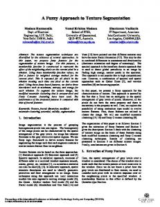
to compare texture analysis methods and one of the best known is the Brodatz database (Brodatz, 1966). In (Kopf et al., 2007), Johannes Kopf et al construct solid textures from two-dimensional texture images. Some examples are available 1 but currently there are too few images to make a classification experiment. In (Gool et al., 1985), Van Gool et al describe three classes of texture with deterministic textures, stochastic textures and observable textures. The first category is characterized by the repetition of a geometrical pattern. This kind of texture can be synthesized using a pattern of specific size and direction. To the contrary, stochastic textures are irregular and no repetitive pattern is identifiable. At last observable textures can be defined as a mix between geometric and stochastic textures. Patterns are very closed but not identical. To have a complete and representative database, we have tried to build synthetic images representative of all these three classes. To limit necessary disk space and processing time, each of the volumetric texture images have a size of 643 . This size seems sufficient to allow classification experiments. The images have been constructed using four different methods. With a first method, volumetric textured images are constructed using two-dimensional texture images like Brodatz textures, fractal textures etc. Two or more two-dimensional texture images are interpolated to obtain a three dimensional image (Figure 1). It is important to know that two-dimensional textures used to build a three-dimensional image are not exactly similar. With the interpolation, these textures have a particular direction and evolve regularly. A good example of this kind of texture could be a tree bole. An interpolated texture can be defined as a set of textured blocks BT built using two-dimensional textures E: BT,i = ET + i

(ET − ET +1 ) M

solid/textures/index.html

Figure 1: Example of construction of an interpolated solid texture

direction. Moreover, observable texture can be easily generated for example using many sphere with random size and random arrangement. To construct a gruyere texture, we place randomly sphere or ellipsis with random sizes in a yellow three-dimensional image. The properties of this type of texture depends on the number of patterns, the shape of the patterns, the size of patterns which can be fixed or randomly chosen, and the color which can also take a random or fixed value. Figure 2 shows two volumetric textures generated with this method.

(a) Cube Pattern

(1)

with M = N/(R − 1) the number of two-dimensional components in a block, N the depth of the solid texture, R the number of two-dimensional textured images used to interpolate, T = {0, ..., R − 1} and i = {0, 1, ..., M − 1}. The properties of this kind of texture depends on the chosen two-dimensional texture and the number of interpolation plans. A second method consists to use geometric shapes like sphere, cube, ellipsis, etc. With this method it is possible to construct deterministic texture. A pattern will be a geometric shape allocated in a given 1 http://johanneskopf.de/publications/

(a) Two-dimensional textured (b) Volumetric texture by inimages terpolation

(b) Sphere Pattern

Figure 2: Example of solid textures with geometric shapes

The third method allows to synthesize solid texture using Fourier transformation as presented in (Lewis, 1984). For that, it is necessary to construct a power spectrum in order to specify frequencies that will be present in the synthesized texture and their amplitude. It is so possible to paint it with the respect of the quadrant symmetry or using power spectrum from an existing texture. For the phase spectrum, we can use random value or take it from an existing texture. Then, we are able to synthesize solid textures with an inverse Fourier transform using these two components. Each example of texture in a given class is not exactly similar. Indeed, examples in a class are made using a unique power spectrum and a phase spectrum with

(a) Power Spectrum 1

(b) Texture build with the first power spectrum

(c) Power Spectrum 2

(d) Texture build with the second power spectrum

Figure 5: [a-c]) Solid textures with random rotation, [d-e] Two blurry textures, [f-g] Two noisy textures, [h-i] Two subsampled textures

Figure 3: Example of solid textures build using inverse Fourier transform

some variations. As describe in (Lewis, 1984), this texture synthesize method is not intuitive, but allows to construct rich textures difficult to obtain in the spatial domain. At last, it is also possible to obtain a fourth category of three-dimensional images using a mix between the three previous methods. Instead of generate a pattern with a color like in the second method, we can create patterns with a given texture using the first synthesis method or texture obtained with the inverse Fourier transform (Figure 4). The textures

so generated contain geometric shapes with a given texture. Moreover it is possible to insert a texture outside patterns to obtain a textured background. A texture like this one is described by the number of pattern, the shape and the size of patterns, and the used texture inside and outside patterns. To complete this database, we apply some transformations on each class of texture with rotations according x, y and z axis. This is so possible to test if a texture analysis method is invariant to a given transformation. Moreover, Gaussian noise, Gaussian blur and sub-sampling are applied to increase variability in each existing volumetric texture classes (Figure 5). The interest of using these transformations is to test for example the robustness to noise or blur of an analysis method and to be able to increase easily the difficulty of the comparison between images of the database.

3 (a) Texture Inside Patterns (b) Texture Inside and Outside Patterns Figure 4: Example of solid textures with texture outside or inside geometric shapes

ORGANIZATION OF THE DATABASE

Our database is now available in free access 2 and it is so possible to evaluate volumetric texture anal2 http://www.rfai.li.univ-tours.fr/fr/ressources/

3Dsynthetic_images_database.html

ysis methods with classification experiments or with segmentation problems. The database is organized as follow: each textured images are allocated according to the synthesis method that is to say their are partitioned in four folders. In each folder of texture synthesize type, images are assigned according to the applied distortion: nothing, Gaussian blur, Gaussian noise, rotation or sub sampling. At last, folders of distortion contain examples of the different classes of volumetric textures. Currently, our database contains 95 different classes. 30 of these classes have been built with the interpolation method, 25 with the geometrical shape method, 15 with the inverse Fourier transform and 25 with the blended method. Each class is composed by 50 examples : 10 blurry textures, 10 noisy textures, 10 textures with sub sampling distortion, 10 with random rotations and 10 without any transformation. Each volumetric image is corresponding to a set of 64 gray level BMP images of 64 × 64 pixels stored in a specific directory. So it is very easy to implement a program able to load such three-dimensional images. A viewer is also available on the web site. We choose to make volumetric textures of size 643 because it is a sufficient size for experiments and this is a good compromise for disk storage. At last, images for segmentation experiments (images that contain more than one texture) have a size of 1283 that allows a better degree of freedom to emplace textures. For each volumetric images, a xml file is generated and contains informations about the image tag. The root of a xml file is an image which can contain one or many solid texture descriptors. Indeed, for a texture recognition problem the used three-dimensional images correspond to an unique solid texture, whereas a three-dimensional image contains more than one volumetric texture for a segmentation problem. A solid texture is defined by a packaging, a name which correspond to the name of a class, the type of synthesis used, properties and distortions which have been applied. A packaging is used because in the case of a segmentation problem, a volumetric texture is not automatically defined in a cube. Currently, a texture can be created according to three different shapes (cube, sphere, ellipsis), with a given size, a given location and with a particular orientation. Properties depend on the type of synthesize method used to make a texture as describe in section 2. For example, a volumetric texture made with inverse Fourier transform depends on the input power spectrum. In order to utilize these xml files we made a DTD file (appendix) which is available in our web site. In this section, we describe the structure of our database. Each images is described by a xml data

and a DTD specify the formalism. Using this DTD, it is then possible for a researcher to complete this database with its proper methods or with an existing one in order to increase the number of classes and images. Currently the database contains 95 different classes which is enough if we compare with existing two-dimensional databases. For example Brodatz database (Brodatz, 1966), which is a standard for evaluating texture algorithms, has 112 different classes.

4

EXPLOITATION OF THE DATABASE

This part is a description of different ways to exploit our database. We have seen that two types of images are available: images containing one solid texture and images with multiple solid textures. Threedimensional images with single volumetric texture can be used to create a classification problem. Here the purpose is that the tested classification algorithms decide which is the class of a texture. Images with many solid texture allow to test methods for classification (a label is attributed to a voxel) or segmentation. Image segmentation and recognition are two aspects of the same problem: in the first case an image is divided into homogeneous zones delimited by boundaries whereas classification consists in labeling or indexation of components (image,voxel etc.). A lot of methods have been proposed for the evaluation of segmentation and classification algorithms (Zhang, 1996). Here we will review some of them to explain how to evaluate an algorithm with our database.

4.1

Classification evaluation

We have seen that the goal of a classification method is to decide the class of a given image. In general, a classification system can be divided in three step. The first one consist to extract features from the images. In the case of texture problem, it is used classical algorithms which have been quickly presented in our introduction (Haralick et al., 1973; Chellappa and Jain, 1993; Mallat, 1989; Ojala et al., 1996). The second one consist in a selection of features. This step allows to reduce the feature space and to keep the most significant features for an application. In the last one, feature vectors are used to feed classification algorithms like for example neural network, support vector machine, k-nearest neighbors etc. To classify images with these algorithms, there are two important stages: a learning phase which uses a learning database and a test phase which is applied on a

test database. In the first phase, a classification algorithm learns features which correspond to the different classes and during the second one, we just test how the classification algorithm tags the different images. To evaluate classification systems and compare their robustness in a given application, a classical approach is the confusion matrix which represent the number of elements ci, j from the class i classified in the class j. The normalized confusion matrix NCM can be computed as follow: ci, j NCMi, j = T (2) ∑k=1 ci,k with T the number of considered classes. Using this matrix, it is then possible to compute some measures like: the true positive rate, T Pratei = NCMi,i false positive rate, T

FPratei =

∑

(4)

NCMi, j

j=1, j6=i

accuracy, ∑Ti=1 NCMi,i T error classification rates ECR with for example: Accuracy =

0.5(∑Tj=1, j6=i NCMi, j + ∑Tj=1, j6=i T i=1 T

ECR = ∑

Figure 6: Example of an ROC graph

(3)

(5)

NCM j,i T −1 )

(6) In this error classification rate, we consider two errors with elements from a given class i falsely classified as elements of another class and elements classified in a given class j but belonging to an other class i. In (Martin et al., 2006), Martin et al propose an interesting approach which consists to make a confusion matrix taking into account the inhomogeneous units and uncertain of the experts. This method can be interesting in the case of natural images which usually require more than one expert classification. Another way to examine the performance of classifiers is to use a receiver operating characteristics (ROC) graph which is a technique for visualizing and selecting classifiers based on their performance. ROC graphs are two-dimensional graphs where Y axis represents T Prate (formula 3) and where FPrate (formula 4) is plotted on the X axis. For a given class, an ROC graph describes trades off between true positive and false positive. Then, if T classes are considered, it is possible to generate T different ROC graphs. For each classifier, we can compute a (FPrate, T Prate) pair that allows to compare their performance (Figure

6). The point (0, 1) which correspond to C classifier represents perfect classification. For more information about ROC analysis, Fawcett in (Fawcett, 2006) presents a guide for using them in research in order to promote better evaluation practices. Their exist several measure to evaluate classification problems. In (Ferri et al., 2008), Ferri et al describe and study the relationships between the most common performance measures for classifiers. They conclude about the existence of important similarities between measures but also significant differences between others.

4.2

Segmentation evaluation

As explain in (Martin et al., 2006), method like confusion matrix allows only an evaluation of the classification approach but does not give an evaluation of the produced segmentation. Segmentation evaluation can not be made by visual comparison but using some metrics. Some methods have been proposed and can be classified in two families: supervised evaluation methods that require access to a ground truth reference and unsupervised evaluation methods that do not have an a priori knowledge of the correct segmentation. Supervised evaluation methods measure the degree of similarity between expert and machine segmentation. The main advantage of this kind of methods is that they allows to obtain a very fine resolution of the evaluation. Nevertheless, generate a ground truth can be difficult and cost a lot of time. It is not the case with our database. Indeed segmented images are available and it is easy to construct them using informations in xml files (figure 7). To evaluate a

segmentation, it is necessary to take into account different possible errors: under-segmentation where components are missing, over-segmentation which correspond to an addition of pixel in a contour, and localisation errors. In (Chabrier et al., 2008), Chabrier et al propose a comparative study of 14 supervised evaluation criteria according to several degradations (under-segmentation, over-segmentation etc.). Their conclusion is that the Pratt criterion is the most effective and allows more discriminated results.

Unsupervised evaluation methods are quantitative and objective evaluation and require no reference image. These kind of method are very interesting because for many applications it is sometimes impossible or very difficult to provide a reference image. For example generate a ground truth for threedimensional ultrasound images is a problem because of their complexity and the third dimension. A lot of metrics have been presented and some of them propose for example to measure intra-region uniformity, inter-region disparity, the shape etc. In (Zhang et al., 2008), Zhang et al propose a survey of these unsupervised methods and present experiments to evaluate them along different situations.

5

CONCLUSIONS

In this paper, we propose a solid texture database for the evaluation and comparison of volumetric texture classification and segmentation methods. Different approaches have been used to obtain images with a wide variety of textures. The first method makes solid textures by interpolating two-dimensional images, the second method by using geometric shapes like sphere, ellipsis or cube, the third one by applying the inverse Fourier transform to a given power spectrum and the last one by generating shapes with a particular texture. Furthermore, different sets of images have been produced by adding different types of distortions. Two types of images are available: images with one solid texture and images with multiple solid textures. Each of them is described by a xml data and a DTD specify the formalism. It is then possible for a researcher to complete this database with other methods. At last, we explain different ways to exploit our database with a description of common evaluation methods. Currently, this database is in free access and it is possible to test texture analysis methods for classification and segmentation purpose. At last it could be interesting to complete this database and provide some natural images like three-dimensional medical images.

REFERENCES

(a) Original image

(b) Uniform region

(c) Corresponding boundaries

Figure 7: Example of a three-dimensional image with three solid textures and its corresponding ground truth

Brodatz, P. (1966). Textures: A Photographic Album for Artists and Designer. Dover Pub. Chabrier, S., Laurent, H., Rosenberger, C., and Emile, B. (2008). Comparative study of contour detection evaluation criteria based on dissimilarity measures. EURASIP Journal on Image and Video Processing, 2008:13 pages. Chellappa, R. and Jain, A. K. (1993). Markov Random Fields Theory and Application. Academic Press. Cuba, O. and Dana, K. (2004). 3d texture recognition using bidirectional feature histograms. International journal of Computer Vision, 59(1):33–60. Fawcett, T. (2006). An introduction to roc analysis. Pattern Recognition Letters, 27:861–874. Ferri, C., Orallo, J. H., and Modroiu, R. (2008). An experimental comparison of performance measures for classification. Pattern Recognition Letters. Gool, L. J. V., Dewaele, P., and Oosterlinck, A. (1985). Texture analysis anno 1983. Computer Vision, Graphics, and Image Processing, 29(3):336–357. Haralick, R. M. (1979). Statistical and structural approaches to textures. Proceedings of the IEEE, 67(5):786–804. Haralick, R. M., Shanmugam, K., and Dinstein, I. (1973). Texture features for image classification. IEEE Transactions on Systems, Man and Cybernetics, 3(6):610– 621.

Jafari-Khouzani, K., Soltanian-Zadeh, H., Elisevich, K., and Patel, S. (2004). Comparison of 2d and 3d wavelet features for tle lateralization. In Proceedings of the SPIE, volume 5369. Julesz, B. (1962). Visual pattern recognition. IEEE Transaction on Information Theroy, 8. Kopf, J., Fu, C.-W., Cohen-Or, D., Deussen, O., Lischinski, D., and Wong, T.-T. (2007). Solid texture synthesis from 2d exemplars. In SIGGRAPH ’07: Proceedings of the 34th International Conference and Exhibition on Computer Graphics and Interactive Techniques. Lewis, J.-P. (1984). Texture synthesis for digital painting. SIGGRAPH Computer Graphics, 18(3):245–252. Mallat, S. G. (1989). A theory for multiresolution signal decomposition: the wavelet representation. IEEE transaction on Pattern Analysis and Machine Intelligence, 11:674–693. Martin, A., Laanaya, H., and Arnold-Bos, A. (2006). Evaluation for uncertain image classification and segmentation. Pattern Recogn., 39(11):1987–1995. Mosquera, A., Cabello, D., Carreira, M., and Penedo, M. (1992). A fractal-based approach to texture segmentation. In ICIPA ’92: Proceedings on the International Conference on Image Processing and its Application. Neyret, F. (1995). A general and multiscale model for volumetric textures. In Davis, W. A. and Prusinkiewicz, P., editors, Graphics Interface ’95, pages 83–91. Canadian Information Processing Society, Canadian Human-Computer Communications Society. ISBN 09695338-4-5. Ojala, T., Pietikainen, M., and Harwood, D. (1996). A comparative study of texture measures with classification based on feature distributions. Pattern Recognition, 29(1):51–59. Showalter, C., Clymer, B. D., Richmond, B., and Powell, K. (2006). Three-dimensional texture analysis of cancellous bone cores evaluated at clinical ct resolutions. Osteoporos International, 17:259–266. Suzuki, M. T., Yoshitomo, Y., Osawa, N., and Sugimoto, Y. (2004). Classification of solid textures using 3d mask patterns. In ICSMC ’04: International Conference on Systems, Man and Cybernetics. Tuceryan, M. and Jain, A. K. (1990). Texture segmentation using voronoi polygons. IEEE Transactions On Pattern Analysis And Machine Intelligence, 12:211–216. Tuceryan, M. and Jain, A. K. (1998). Texture Analysis, chapter 2.1, pages 207–248. The Handbook of Pattern Recognition and Computer Vision. Zhang, H., Fritts, J. E., and Goldman, S. A. (2008). Image segmentation evaluation: A survey of unsupervised methods. Computer Vision and Image Understanding, 110:260–280. Zhang, Y. (1996). A survey on evaluation methods for image segmentation. Pattern Recognition, 29(8):1335– 1346.

APPENDIX In this appendix we present the main components of our DTD. To obtain the complete DTD, it is possible to download it using our website. ————————————————————– ... ————————————————————– ————————————————————– ————————————————————– ... ... ... ... ... ————————————————————– ... ————————————————————–