Abstract. In this study we present a new sparse polynomial regression mixture model for fitting time series. The contribution of this work is the introduction of a ...
A sparse regression mixture model for clustering time-series K. Blekas and N. Galatsanos and A. Likas Department of Computer Science, University of Ioannina, 45110 Ioannina, Greece E-mail: {kblekas, galatsanos, arly}@cs.uoi.gr
Abstract. In this study we present a new sparse polynomial regression mixture model for fitting time series. The contribution of this work is the introduction of a smoothing prior over component regression coefficients through a Bayesian framework. This is done by using an appropriate Student-t distribution. The advantages of the sparsity-favouring prior is to make model more robust, less independent on order p of polynomials and improve the clustering procedure. The whole framework is converted into a maximum a posteriori (MAP) approach, where the known EM algorithm can be applied offering update equations for the model parameters in closed forms. The efficiency of the proposed sparse mixture model is experimentally shown by applying it on various real benchmarks and by comparing it with the typical regression mixture and the K-means algorithm. The results are very promising. Keywords: Clustering time-series, Regression mixture model, sparse prior, Expectation-Maximization (EM) algorithm.
1
Introduction
Clustering is a very interesting and challenging research problem and a wide spectrum of methodologies has been used to address it. Probabilistic mixture modeling is a well established model-based approach for clustering that offers many advantages. One such advantage is that it provides a natural platform to evaluate the quality of the clustering solution [1], [2]. Clustering time-series is a special case of clustering in which the available data have one or both of the following two features: first they are of very large dimension and thus conventional clustering methods are computationally prohibitive, and second they are not of equal length and thus conventional clustering methods cannot straightforwardly be applied. In such cases it is natural initially to fit the available data with a parametric model and then to cluster based on that model. Different types of functional models have been used to for such data. Among them polynomial and spline regression are the most commonly used models [3] and have been successfully applied to a number of diverse applications, ranging from gene clustering in bioinformatics to clustering of cyclone trajectories, see for example [4] [5], [6] and [7].
Sparse Bayesian regression is methodology that has received a lot of attention lately, see for example [8], [9], [10] and [11]. Enforcing sparsity is a fundamental machine learning regularization principle and lies behind some well known subjects such as feature selection. The key idea behind sparse priors is that we can obtain more flexible inference methods by employing models with many more degrees of freedom than could uniquely be adapted given data. In particular, the target of sparse Bayesian regression is to impose a heavy tail priors to the coefficients of the regressor. Such prior will zero out the coefficients that are not significant and maintain only a few large coefficients that are considered significant based on the model. The main advantage of such models is that they address the problem of model order selection which is a very important problem in many model based applications including regression. If the order of the regressor model is too large it overfits the observations and does not generalize well. On the other hand if it is too small it might miss trends in the data. In this paper we present a sparse regression mixture model for clustering timeseries data. It is based on treating the regression coefficients of each component as Gaussian random variables, and sequentially the inverse of their variance as Gamma hypepriors. These two hierarchical priors constitute the Student-t distribution which has been proved to be very efficient [8]. Then, a maximum a posteriori expectation maximization algorithm (MAP-EM) [12], [2] is applied to learn this model and cluster the data. This is very efficient since it leads to update rules of model parameters in closed form during the M -step and improves data fitting. The performance of the proposed methodology is evaluated using a variety of real datasets. Comparative results are also obtained using the classical K-means algorithm and also the typical regression mixture model without the sparse prior. Since the ground truth is already known, we have used the percentage of correct classification for evaluating each method. As experimentally have shown, the main advantage of our method is through sparsity property to achieve more flexibility and robustness with better solutions. In section 2 we present the simple polynomial regression mixture model and how the EM algorithm can be used for estimating its parameters. The proposed sparse regression method is then given in section 3 describing the sparse Studentt prior over the component regression coefficients. To assess the performance of the proposed methodology we present in section 4 numerical experiments with known benchmarks. Finally, in section 5 we give our conclusions and suggestions for future research.
2
Regression Mixture Models
Suppose the set of N time-series data sequences Y = {yil }l=1,...,T i=1,...,N , where l denotes the temporal index that corresponds to time locations tl . It must be noted that although during the present description of the regression model it is assumed that all yi sequences are of equal length, this can be easily changed. In
such case, each yi for i = 1, . . . , N is of variable length Ti . This corresponds to the general case of the model. To model time-series yi we use p-order polynomial regression on the time range t = (t1 , . . . , tT ) with an additive noise term given by yi = Xβ + ei , where X is the Vandermonde matrix, i.e. 1 t1 . . . X = ... ... . . .
(1)
tp1 .. .
1 tT . . . tpT
and β is the p + 1-vector of regression coefficients. Finally, the error term ei is a T -dimensional vector that is assumed to be Gaussian and independent over time, i.e. ei ∼ N (0, Σ) with a diagonal covariance matrix Σ = diag(σ12 , . . . , σT2 ). Thus, by assuming Xβ deterministic, we can model the joint probability density of the sequence y with the normal distribution N (Xβ, Σ). In this study we consider the problem of clustering time-series, i.e. the division of the set of sequences yi with i = 1, . . . N into K clusters, where each cluster will contain sequences of the same generation mechanism (polynomial regression model). To this direction, the regression mixture model is a useful generative model that can be used to capture heterogeneous sources of time-series. This can be described by the following probability density function: f (yi |Θ) =
K X
πj p(yi |θj ) ,
(2)
j=1
which has a generic and powerful meaning in model-based clustering. Following this scheme, each sequence is generated by first selecting a source j (cluster) according to probabilities πj and then by performing sampling based on the corresponding regression relationship with parameters θj = {βj , Σj } as described by the normal density function p(yi |θj ) = N (yi |Xβj , Σj ). Moreover, the unknown PK mixture probabilities satisfy the constraints: πj ≥ 0 and j=1 πj = 1. Based on the above formulation, the clustering problem becomes a maximum likelihood (ML) estimation problem for the mixture parameters Θ = {πj , θj }K j=1 , where the log-likelihood function is given by L(Y |Θ) =
N X i=1
K X
log{
πj N (yi |Xβj , Σj )} .
(3)
j=1
The Expectation-Maximization (EM) algorithm [12] is an efficient framework for solving likelihood estimation problems for mixture models. It performs iteratively two steps: The E-step, where the current posterior probabilities of samples to belong to each cluster are calculated: (t)
(t)
zij = P (j|yi , Θ(t) ) =
(t)
(t)
πj N (yi |Xβj , Σj ) f (yi |Θ(t) )
,
(4)
and the M -step, where the maximization of the expected value of the complete log-likelihood is performed. This leads to the following updated rules for the mixture parameters [4], [3]: N X (t+1)
πj
(t+1) βj
= =
(t)
zij
i=1
N "N X
,
(5) #−1
(t) (t) zij X T Σj−1 X
X T Σj−1
i=1 N X 2 σjl
(t+1)
=
(t)
N X
(t)
zij yi ,
(6)
i=1 (t)
(t+1)
zij (yil − [Xβj
]l ) 2
i=1 N X
,
(7)
(t) zij
i=1
where [.]l indicates the l-th component of the T -dimensional vector that corresponds to location tl . After convergence of the EM, the association of the N observable sequences yi with the K clusters is based on the maximum value of the posterior probabilities. The generative polynomial regression function is also obtained per each cluster, as expressed by the (p + 1)-dimensional vectors of the regression coefficients βj = (βj0 , βj1 , . . . , βjp )T .
3
Sparse Regression Mixture Models
An important issue, when using the regression mixture model is to define the order p of the polynomials. The appropriate value of p depends on the shape of the curve to be fitted. Polynomials of smaller order lead to underfitting, while large values of p may lead to curve overfitting. Both cases may lead to serious deterioration of the clustering performance as also verified by experimental results. The problem can be tackled using some regularization method that penalizes large order polynomials. An elegant statistical method for regularization is the Bayesian approach. This technique assumes a large value of the order p and imposes a prior distribution p(βj ) on the parameter vectors (βj0 , βj1 , . . . , βjp )T of each polynomial. More specifically, the prior is defined in a hierarchical way as follows: p(βj |αj ) = N (βj |0, A−1 j )=
p Y
−1 N (βk |0, αjk )
(8)
k=0
where N (µ|0, Σ) is the normal distribution and Aj is a diagonal matrix containing the p + 1 elements of the hyperparameter vector αj = [αj0 . . . αjp ].
In addition a Γ prior is also imposed on the hyperparameters αjk : p(αj ) =
p Y
Gamma(αjk |a, b) ∝
k=0
p Y
a−1 −bαjk αjk e ,
(9)
k=0
where where a and b denote parameters that are a priori set to near zero values. The above two-stage hierarchical prior on αj is actually a Student-t distribution and is called sparse ([8]), since it enforces most of the values αjk to be large, thus the corresponding βjk are set zero and eliminated from the model. In this way the complexity of the regression polynomials is controlled in an automatic and elegant way and overfitting is avoided. This prior has been successfully employed in the Relevance Vector Machine (RVM) model [8]. In order to exploit this sparse prior we resort to the MAP approach where the log-likelihood of the model (Eq. 3) is augmented with a penalty term that corresponds to the logarithm of the prior p(βj ). L(Y |Θ) =
N X
log{
i=1
K X
πj N (yi |Xβj , Σj )} +
j=1
K X
log p(βj |αj ) +
j=1
K X
log p(αj ) (10)
j=1
where the parameter vector Θ is augmented to include the parameter vectors aj : Θ = {πj , βj , Σj , αj }K j=1 . Maximization of the MAP log-likelihood with respect to the parameters Θ is again achieved using the EM algorithm. At each EM iteration t, the computation of the posteriors zij in the E-step is again performed using Eq. (4). The same happens in the M-step for the update of the parameters πj and Σj which is performed using Eq. (4) and Eq. (6). The introduction of the sparse prior affects the update of the parameter vectors βj which is now written as: " (t+1) βj
=
N X
#−1 (t) (t) zij X T Σj−1 X
+
(t) Aj
X T Σj−1
i=1
(t)
N X
(t)
zij yi ,
(11)
i=1
while the update of the hyperparameters αjk is given by: (t+1)
αjk
=
2a − 1 (t+1) βjk
+ 2b
(12)
In the last equation the values of a and b have been set to 10−4 . It must be noted that at each M-step, in order to accelerate convergence, it possible to iteratively apply the update equations for βj and αjk more than once. In our experiments two update iterations were carried out.
4
Experimental Results
We have made experiments on a variety of known benchmarks in order to study the performance of the proposed sparse regression mixture model, referred as
Sparse RM. Comparative results were obtained with the typical regression mixture model, that will be referred next as Simple RM. Both methods were initialized with the same strategy. In particular, at first K time-series are randomly selected form the dataset for initializing the polynomial coefficients βj of the K components of the mixture model, following the simple least-square fit solution. Then, the log-likelihood function value is calculated after performing one step of the EM algorithm. One hundred (100) such different one-EM-step executions are made and the parameters of the model that capture the maximum likelihood value are finally used for initializing the EM algorithm. Table 1. The description of the five datasets used in our experimental study. Dataset Number of classes (K) Size of dataset (N ) Time series length (T ) CBF 3 930 128 ECG 2 200 96 Gun problem 2 200 150 Synthetic control 6 600 60 Trace 4 200 275
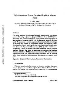
In Table 1 we present some characteristics (the size and the number of classes) of the five (5) real datasets we have used in our experimental study. In particular, we have selected five (5) datasets for evaluating our method [13]: – The Cylinder-Bell-Funnel (CBF) dataset contains time series from three different classes generated by three particular equations, see [14]. – The ECG dataset characterized by underlying patterns of periodicity. – The Gun problem comes from a video surveillance domain that gives the motion streams from the right hand of two actors. – The Synthetic control dataset which comes from monitoring and control of process environments. – The Trace dataset which is a synthetic dataset designed to simulate instrumentation failures in nuclear plant. More details on these benchmarks can be found at [13]. The obtained results from the comparative study on these benchmarks are summarized in Figure 1. For each one of the five problems we present a diagram with the accuracy of both methods for various values of polynomial order p. Note that we present here the mean values of the correct classification percentage as obtained from twenty (20) runs per order value. Furthermore, these diagrams illustrate (grey straight lines) the performance of the K − means algorithm, where the time series are treated as feature vectors. It must be noted that these results are published in [13] and correspond to the best solution found after 10 different runs of the K-means. As it is obvious from the diagrams of Figure 1 the typical regression model (Simple RM) deteriorate the clustering performance, especially in cases of large
ECG dataset
CBF dataset 80
75
75
70
70
65 accuracy (%)
accuracy (%)
65 60 Sparse RM Simple RM K−means
55 50 45
Sparse RM Simple RM K−means
60 55 50
40
45
35 30
2
4
6
8
10
12
14
16
18
40 0
20
2
4
6
8
order p Gun dataset
14
16
18
20
Synthetic control dataset
68
80 Sparse RM Simple RM K−means
66 64
70 60 accuracy (%)
62 accuracy (%)
10 12 order p
60 58 56 54
Sparse RM Simple RM K−means
50 40 30
52 20
50 48
2
4
6
8
10
12
14
16
18
10
20
2
4
6
order p
8
10
12
14
16
18
20
order p Trace dataset 60
Sparse RM Simple RM K−means
58
accuracy (%)
56 54 52 50 48 46 44 42
2
4
6
8
10
12
14
16
18
20
order p
Fig. 1. Comparative results from the experiments on five benchmarks. The mean value of the correct classification for each one of the three methods is illustrated for different values of the polynomial order p.
polynomial order p values, leading in strong overfitting in all experimental datasets. On the other hand, the proposed sparse regression mixture model has the ability to overcome this disadvantage with the use of the sparsity potential, and to maintain better performance throughout the range of the polynomial order p. Therefore, it seems that the availability of sparsity makes the clustering approach independent on the polynomial order. Furthermore, that is more interesting is that in most cases, such as in the CBF, the ECG and the Trace datasets (Figure 1), the best clustering solution was obtained for large values of order p, where the typical RM completely fails. This is of great advantage, since it may lead to improve the model generalization ability. Thus, we recommend the use of sparse regression mixture model with a large polynomial order value (e.g. p = 15) and allow the model to select the most useful among the regression coefficients and sets to zero the rest of them.
5
Conclusions and Future Work
In this paper we presented an efficient methodology for clustering time-series, where the key aspect of the proposed technique is the sparsity of the regression polynomials. The main scheme applied here is the polynomial regression mixture model. Adding sparsity to the polynomial coefficients introduces a regularization principle that allows to start from an overparameterized model and force regression coefficients close to zero if they are not useful. Learning in the proposed sparse regression mixture model is treated in a maximum a posteriori (MAP) framework that allows the EM algorithm to be effectively used for estimating the model parameters. This has the advantage of establishing update rules in closed form during the M -step and thus data fitting can be done very efficiently. Experiments on difficult datasets have demonstrated the ability of the proposed sparse models to improve the performance and the robustness of the typical regression mixture model. Our further research on this subject is mainly focused on three directions. In particular, we can alternatively use another design matrix X for regression (Eq. 1), apart from the simplest Vandermonde matrix in the case of polynomial. Following the Relevance Vector Machine (RVM) approach [8], different types of Kernel matrices can be examined, such as Gaussian Kernel. On the other hand, we are planning to examine also the possibility of using another type of more advantageous sparse priors, such as those presented at [10], [11] that have recently applied to general linear sparse models. The third target of our future work is to eliminate the dependence of the proposed regression mixture model on the initialization. Experiments have shown that in some cases there is a significant dependence on initializing model parameters especially on the regression parameters βjk . A possible solution is to design an incremental procedure for learning a regression mixture model by adopting successful schemes that have already been presented in the case of classical mixture models [15]. Finally, we are planning to study the performance of the proposed methodology and its ex-
tensions in computer vision applications, such as visual tracking problems and object detection in a video surveillance domain [16], [17].
References 1. C.M. Bishop. Pattern Recognition and Machine Learning. Springer, 2006. 2. G. M. McLachlan and D. Peel. Finite Mixture Models. New York: John Wiley & Sons, Inc., 2001. 3. S. J. Gaffney and P. Smyth. Curve clustering with random effects regression mixtures. In C. M. Bishop and B. J. Frey, editors, Proc. of the Ninth Intern. Workshop on Artificial Intelligence and Statistics, 2003. 4. W. S. DeSarbo and W. L. Cron. A maximum likelihood methodology for clusterwise linear regression. Journal of Classification, 5(1):249–282, 1988. 5. D. Chudova, S. Gaffney, E. Mjolsness, and P. Smyth. Mixture models for translation-invariant clustering of sets of multi-dimensional curves. In Proc. of the Ninth ACM SIGKDD Intern. Conf. on Knowledge Discovery and Data Mining, pages 79–88, Washington, DC, 2003. 6. S. J. Gaffney. Probabilistic curve-aligned clustering and prediction with regression mixture models. PhD thesis, Department of Computer Science, University of California, Irvine, 2004. 7. K. Blekas, C. Nikou, N. Galatsanos, and N. V. Tsekos. A regression mixture model with spatial constraints for clustering spatiotemporal data. Intern. Journal on Artificial Intelligence Tools (to appear). 8. M. E. Tipping. Sparse Bayesian Learning and the Relevance Vector Machine. Journal of Machine Learning Research, 1:211–244, 2001. 9. M. Zhong. A Variational method for learning Sparse Bayesian Regression. Neurocomputing, 69:2351–2355, 2006. 10. A. Schmolck and R. Everson. Smooth Relevance Vector Machine: A smoothness prior extension of the RVM. Machine Learning, 68(2):107–135, 2007. 11. M. Seeger. Bayesian Inference and Optimal Design for the Sparse Linear Model. Journal of Machine Learning Research, 9:759–813, 2008. 12. A. P. Dempster, N. M. Laird, and D. B. Rubin. Maximum Likelihood from incomplete data via the EM algorithm. J. Roy. Statist. Soc. B, 39:1–38, 1977. 13. E. Keogh, X. Xi, L. Wei, and C.A. Ratanamahatana. The ucr time series classification/clustering homepage: www.cs.ucr.edu/∼eamonn/time series data/, 2006. 14. E. J. Keogh and M. J. Pazzani. Scaling up Dynamic Time Warping for Datamining Applications. In 6th ACM SIGKDD International Conference on Knowledge Discovery & Data Mining, pages 285–289, 2000. 15. N. Vlassis and A. Likas. A greedy EM algorithm for Gaussian mixture learning. Neural Processing Letters, 15:77–87, 2001. 16. O. Williams, A. Blake, and R. Cipolla. Sparse Bayesian Learning for Efficient Visual Tracking. IEEE Trans. on Pattern Analysis and Machine Intelligence, 27(8):1292–1304, 2005. 17. G. Antonini and J. Thiran. Counting pedestrians in video sequences using trajectory clustering. IEEE Trans. on Circuits and Systems for Video Technology, 16(8):1008–1020, 2006.