diagram. The required perceptions and actions are defined in terms of .... Actions Given a finite set C of spatial constraints defined on a diagrammatic object o ... The VR Behind(q, a, p) returns True iff .... our inputs are closer to the problem statements and do not suggest any solution .... For the analytic proof, the statement of ...
Appears in Proc. 1st International Workshop on Constraint Programming for Graphical Applications. In conjunction with 12th International Conference on Principles and Practice of Constraint Programming, Nantes, France, September 24-30, 2006.
A Spatial Constraint Satisfaction Framework for Synthesizing Perceptions and Actions in Diagrammatic Reasoning? Bonny Banerjee and B. Chandrasekaran Laboratory for AI Research, Department of Computer Science and Engineering The Ohio State University, Columbus, OH 43210, USA {Banerjee | Chandra}@cse.ohio-state.edu
Abstract. Diagrammatic reasoning is often modeled as a process in which subtasks may be solved, as appropriate, either by inference from symbolic representations or by information extracted by perception from a diagram, and additional subtasks may create or modify objects in the diagram. The required perceptions and actions are defined in terms of properties and relations to be satisfied by a set of diagrammatic objects. Performing such perceptions and actions in general requires visual problem solving for humans. This paper investigates the use of spatial constraint satisfaction for automatically synthesizing solutions for perceptions and actions. Our research goal is to develop a high-level language that is finite, extensible, human-usable, and expressive enough to describe the properties of desired perceptions and actions as constraints specified in terms of well-defined mathematical/logical functions and predefined perceptions/actions; to compute the solutions of the desired perceptions/actions and diagrammatically represent the outcome for actions; and to automatically synthesize their programs, thereby transforming them into readily executable routines. The ideas are illustrated by several examples in different domains.
1
Introduction
AI models problem solving as a search for a path to a goal state from an initial state. Traditionally, the underlying representations have been in the so-called symbolic framework, i.e. the goal, the states and the operators that transform the states are all represented as compositions of predicate-symbolic structures, similar to natural language. However, in real-world problem solving, states and operators often have perceptual components, such as when diagrams are used in problem solving. In diagrammatic reasoning (DR), problem solving proceeds opportunistically. In addition to the traditional symbolic state transformations, perception may be called upon to extract certain information from the diagram, ?
This research was supported by participation in the Advanced Decision Architectures Collaborative Technology Alliance sponsored by the U.S. Army Research Laboratory under Cooperative Agreement DAAD19-01-2-0009.
Routines: Abstraction /Visual /Action
Problem Solver
External Diagram Inference Rules Internal Diagram
Symbolic Information
Fig. 1. Role of perception, action and abstraction in a DR architecture.
or actions may be taken on the diagram to create or modify parts of it to satisfy a given description. For example, a problem solving episode might need the information whether there exists a school within five miles from the agent’s home. This might require that the agent automatically abstract his home and all schools in a given map as points and apply appropriate perception operations to extract the required information. In this paper, we concentrate on how an artificial problem-solving agent might perceive from or act on a diagram. In the last couple of decades, numerous DR systems have been built for different purposes, such as analyzing structural problems in civil engineering [1], assisting in geometry theorem proving [2], mathematical theorem proving [3], understanding juxtaposition diagrams of physical situations [4], reasoning about military courses of action [5, 6], and so on. A common requirement of all these systems is the ability to obtain information about spatial properties and relations from a diagram and to modify or create diagrammatic objects (see Fig.1). These abilities have been referred to as routines, as in humans with repeated applications they eventually become so hardwired that they can be performed as a prescribed sequence of operations with limited problem solving. In DR, the perception abilities are called Visual Routines (VRs) while the modification/creation abilities are called Action Routines (ARs). However, synthesizing VRs and ARs from their definitions in terms of properties and relations satisfied by a set of diagrammatic objects requires problem solving. We approach the problem of automatically synthesizing VRs/ARs as having three components – to develop a high-level language that is finite, extensible, human-usable, and expressive enough to describe the properties of desired VRs and ARs as constraints specified in terms of well-defined mathematical/logical functions and predefined VRs/ARs; to symbolically compute the desired VRs/ARs and dia-
grammatically represent an instance of the object if produced as the outcome; and to automatically synthesize their programs. For an artificial problem-solving agent, we define a diagram as an abstract data-structure consisting of a set of labeled primitive objects, whose spatiality is relevant to reasoning, along with their spatial information. Our experimental results are illustrated using examples of VRs/ARs applied to diagrams that are monochromatic with no intensity variation and are configurations of three primitive kinds of objects - points, curves, regions.
2
The Framework
We propose a functional constraint logic programming language for defining VRs and ARs, a framework of spatial constraint satisfaction for automatically computing the solution for a VR/AR from its definition and diagrammatically represent an instance of the solution, and a generic constraint solver for VR/AR program synthesis. The framework supports diagrams in the form of pixel/arraybased and geometric/topological representations. 2.1
Language for expressing VRs/ARs
Programming in a functional language has several advantages. The programs are concise, modular, and have clean semantics. Constraint logic programming has built-in efficient and sound system of equation solvers and the means to perform programmed search implicit in the language itself. The factors of concern to us for choosing the language for defining VRs/ARs are – development time and effort, flexibility in adaptation of the system to other domains or in accepting knowledge from a user, and facilities available in the language itself suitable for problem solving. VRs/ARs can be defined and computed using systems of operations research, genetic algorithms, simulated annealing, etc. but such programs cannot be updated dynamically. Conventional programs can potentially give the most computationally efficient solution, but this requires an uphill development phase which includes tailoring the programs (data-structures, search strategies, etc.) for the particular application thereby making them not readily adaptable to other scenarios. Rule-based languages lack constraint solving capabilities. Constraintbased approaches are flexible to adaptation and receptive to additional knowledge from the user. For particular problems, the efficiency might not be as good as handcrafted conventional programs but still are pretty good due to the presence of very efficient internal constraint solving algorithms, and can deal with sizeable problems exhibiting a reasonably good performance. We consider points, curves, regions as primitive diagrammatic objects in our framework. A point is represented as a pair of coordinates, a curve as a sequence of points joined by piecewise linear segments, while a region as a set of equations and inequalities depicting the points inside a closed curve. A line segment is represented by its parametric equations.
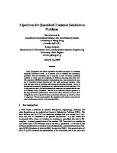
Fig. 2. The shaded region r is behind a curve c with respect to a point p.
2.2
Computing VRs/ARs as spatial constraint solving
While spatial constraint solving has been extensively used for geometry theorem proving [7] and computer-aided design [8] for the last few decades, and more recently to origami construction, application of the same for automatically computing VRs/ARs is a novel idea, which requires handling arbitrary objects and solving hard perceptual problems. Perceptions Given a finite set O of diagrammatic objects and a finite set C of spatial constraints defined on them, a VR returns T rue if O satisfies C, otherwise returns F alse. For example, the VR Collinear(p, q, r) returns T rue iff the points p, q, r lie on a straight line, i.e. p.y−q.y Collinear(p, q, r) = ( p.x−q.x r.x−q.x == r.y−q.y ) A VR might also return a real number when it computes a property involving the objects in O that satisfy C. For example, the VR Distance(p, q) returns the Euclidean distance between two points p, q, i.e. p Distance(p, q) = (p.x − q.x)2 + (p.y − q.y)2 Again, a VR might return a diagrammatic object that emerges due to the objects in O satisfying certain constraints. For example, the VR IntersectionP t(c1 , c2 ) returns the point(s) of intersection of two curves c1 , c2 , i.e. IntersectionP t(c1 , c2 ) = {q : isaP oint(q) ∧ On(q, c1 ) ∧ On(q, c2 )} Thus, formally a VR f might be defined as a mapping from a set of diagrammatic objects O satisfying a set of constraints C to a set of booleans {T rue, F alse} or real numbers < or diagrammatic objects O0 , i.e. f : O → {T rue, F alse} ∪ < ∪ O0 Actions Given a finite set C of spatial constraints defined on a diagrammatic object o, an AR determines whether there actually exists none, one or many
instances of the object o that satisfy C, and returns the spatial properties (extent and location) of the satisfying objects. For example, the AR BehindCurve(p, c), where p is a point and c is a curve, is defined as the set of all points that lie behind c with respect to p (see Fig.2). The VR Behind(q, a, p) returns True iff the point q is behind point a with respect to point p, i.e. q, a, p are collinear and a lies between q and p. Thus, BehindCurve(p, c) = {q : isaP oint(q) ∧ ∀a, isaP oint(a) ∧ On(a, c) ⇒ Behind(q, a, p)} On(a, c) = (∃t, c.x(t) == a.x ∧ c.y(t) == a.y) Behind(q, a, p) = (Collinear(q, a, p) ∧ Between(a, q, p)) a.y−q.y Between(a, q, p) = (0 ≤ a.x−q.x p.x−q.x ≤ 1 ∨ 0 ≤ p.y−q.y ≤ 1) Abstractions In DR, a set of diagrammatic objects are often abstracted to more suitable objects depending on the problem solving goals in order for reasoning to proceed in an opportunistic and computationally efficient manner. For example, a bunch of points in a plot is abstracted as a curve to understand the nature of how a variable depends on another. Given a set of points S and a set of models of curves M , the abstraction routine AbstractCurve(S, M ) computes the parameters for the model that minimizes the regression error, i.e. m X AbstractCurve(S, M ) = {Q : Q ∈ M ∧ M inimize( Q(S[i])2 )} i=1
where m is the cardinality of S and S[i] represents the ith element of S. A best curve automatically abstracted using AbstractCurve is shown in Fig.3(a). Another example is the abstraction of a set of points S as an annular region depicting the notion of surrounded. The routine AbstractAnnulus(S) is defined as the region between the smallest circle containing S and the largest circle not containing S but placed entirely inside the points in S. Thus, 2 AbstractSmallestOuterCircle(S) = {{a, b, r} : r ≥ 0 ∧m i=1 ((S[i].x − a) + (S[i].y − b)2 ≤ r2 ) ∧ M inimize(r)} AbstractLargestInnerCircle(S) = {{a, b, r} : M in({S[i].x : 1 ≤ i ≤ m}) ≤ a ≤ M ax({S[i].x : 1 ≤ i ≤ m})∧M in({S[i].y : 1 ≤ i ≤ m}) ≤ b ≤ M ax({S[i].y : 2 2 2 1 ≤ i ≤ m}) ∧m i=1 ((S[i].x − a) + (S[i].y − b) ≥ r ) ∧ M aximize(r)} AbstractAnnulus(S) = {{a1 , b1 , r1 , a2 , b2 , r2 } : {a1 , b1 , r1 } == AbstractSmallestOuterCircle(S) ∧ {a2 , b2 , r2 } == AbstractLargestInnerCircle(S)} An annular region automatically abstracted using AbstractAnnulus is shown in Fig.3(b). Perhaps one of the most widely used abstractions is grouping. We define the routine AbstractnGroups(S, n) as partitioning the set S of points into n groups such that the total variance is minimized. The routine P artition(S, P, i), where P is a set of points, computes the set of points in S that are nearer to the ith point in P than to any other point in P . Thus, #(Q) P artition(S, P, i) = {Q : Q ⊆ S ∧j=1 (∀k, 1 ≤ k ≤ #(P ), i 6= k ⇒ Distance(Q[j], P [i]) < Distance(Q[j], P [k]))}
(a) Curve abstracted from points.
(b) Annular region abstracted from points.
(c) Abstracted groups of points. Fig. 3. Examples of synthesized abstractions.
AbstractnGroups(S, n) = {Q : Q n X M inimize( V ariance(P artition(S, Q, i)))}
⊆
S ∧ #(Q)
==
n ∧
i=1
where #(Q) denotes the cardinality of set Q. Grouping is a NP-hard problem. AbstractnGroups requires searching through a space of O(Cnm ) possible solutions, where m = #(S). The optimum number of groups is obtained by partitioning S into 1, 2,...m groups and by minimizing the product of number of groups and total variance. Thus, AbstractOptGroups(S) = {Q : Q ⊆ {AbstractnGroups(S, i) : 1 ≤ i ≤ i X m} ∧ M inimize(i × V ariance(P artition(S, Q, j)))} j=1
An optimum grouping automatically abstracted using AbstractOptGroups is shown in Fig.3(c). AbstractOptGroups requires searching through a space of O(2m ) possible solutions. 2.3
Program synthesis
Synthesizing solutions for VRs/ARs by constraint solving is in many cases slow due to open ended search, especially in our framework where definitions are closer to the problem specification rather than those for execution. In order to overcome the problem of inefficiency, we store perceptions/actions in the form
of executable symbolic programs delivered from the constraint solvers. These stored programs facilitate the use of perceptions/actions as ”routines” in future. We synthesize and store programs in a functional form with all the constraints reduced such that the output can be readily computed without any problem solving if a specific instance is presented as the input. Also, its form is such that a specific instance of the program can be easily represented in a diagram. This feature is extremely important for debugging purposes. For example, the AR BehindP oint(p1 , p2 ) might be defined as the set of all points with coordinates {x, y} that are behind point p1 with respect to point p2 , i.e. BehindP oint(p1 , p2 ) = {q : isaP oint(q) ∧ Behind(q, p1 , p2 )} In our implementation language, this is written as BehindP oint[p1 , p2 ] = Reduce[Behind[{x, y}, p1 , p2 ], {x, y}, Reals] The synthesized program for the same AR is as follows. 2 y1 +xy2 −x1 y2 BehindP oint[{x1 , y1 }, {x2 , y2 }] = ( x1 y−x2 y−xyx11+x == 0∧((x1 > −x2 x2 ∧ x ≥ x1 ) ∨ (x1 < x2 ∧ x ≤ x1 ))) ∨ (y 6= y2 ∧ ((x 6= 0 ∧ x1 == 0 ∧ x2 == 0 ∧ y1 == y2 ) ∨ (x 6= x2 ∧ x1 == x2 ∧ x2 6= 0 ∧ xx1 y2 2 == y1 ))) where (x1 , y1 ), (x2 , y2 ) are coordinates of the points p1 , p2 respectively. Implementation We use the functional logic programming paradigm supported in Mathematica [9], which has state of the art built-in functions for equation/inequality solving, quantifier elimination, and numerical optimization. The current implementation of our framework has been successful in automatically synthesizing over sixty VRs/ARs in different applications including the ones reported in [10, 2, 3, 5, 6]. We have extensively used the Reduce function in Mathematica that keeps all the possible solutions to a set of equations and inequalities including logical operators and quantifiers. While in principle Reduce can always find the complete solution to any collection of polynomial equations and inequalities with real or complex variables eliminating quantifiers, the results are often very complicated, with the number of components typically growing exponentially as the number of variables increases. The bottleneck of this computation is quantifier elimination, the complexity of which is s(l+1)Π(ki +1) d(l+1)Πki where s is the number of polynomials, their maximum Pdegree is d and coefficients are real, l is the number of free variables while k = ki is the number of quantified variables [11]. Since our inputs are closer to the problem statements and do not suggest any solution strategy, one of our challenges in this research has been to specify the input as simply as possible. While most problems can be defined in multiple ways, we try to select the way that involves the least number of variables. We determine the existence of any conflicting constraints in quadratic time using the method specified in [8].
3
Applications
The proposed framework has been used for a number of applications, namely geometry theorem proving, computer-aided design, mathematical theorem prov-
c2
c1 Fig. 4. Parts of the path c1 inside the shaded region are prone to ambush due to presence of enemies behind c2 .
ing using diagrams, blocks world problems, and military applications. Unlike applications, where the domain is limited to a few objects with nice geometrical properties and relations, problems in military domain require a wide range of objects with arbitrary properties and relations. Thus, choice of such a domain will help us illustrate the expressiveness of the language for defining VRs/ARs and the efficiency of constraint satisfaction framework for computing solutions of VRs/ARs from their definitions. In this paper, we will solve particular versions of two problems – ambush detection and entity re-identification – that are deemed very important due to their frequency of occurrence in the military domain. However, in order to illustrate the versatility of the framework, we will use it to synthesize VRs/ARs for proving theorems and solving problems in geometry. 3.1
Ambush detection
There are two main factors – range of firepower and range of sight – that determine the area covered by a military unit. Presence of terrain features, such as mountains, limit these factors and allow units to hide from opponents. These hidden units not only enjoy the advantage of concealing their resources and intentions from the opponents but can also attack the opponents catching them unawares if they are traveling along a path that is within the sight and firepower range of the hidden units, thereby ambushing them. Thus, it is of utmost importance for any military unit to a priori determine the areas or portions of a path prone to ambush before traversing them. In this application, given a curve or region as a hiding place and the firepower and sight ranges, we show how the regions and portions of path prone to ambush can be automatically computed using the proposed framework. Given a curve c and the firepower and sight range d, we define the AR RiskyRegion(c, d) as the region covered by that range from c. Thus, RiskyRegion(c, d) = {q : isaP oint(q) ∧ ∃a, isaP oint(a) ∧ On(a, c) ∧ Distance(a, q) ≤ d}
The solution of this AR is the shaded region shown in Fig.4 with respect to the curve c2 and a particular value of d. The AR RiskyRegion(r, d) for a region r can be defined by replacing the predicate On(a, c) by Inside(a, r), which is defined as the evaluation of the function r at the point a, i.e. Inside(a, r) = r(a.x, a.y) Given a curve c1 as a path, a curve c2 for hiding, and a range d, we define the AR RiskyP ath(c1 , c2 , d) as parts of c1 covered by that range from c2 i.e. as the set of all points that lie on c1 and also inside the risky region. Thus, RiskyP ath(c1 , c2 , d) = {q : isaP oint(q) ∧ On(q, c1 ) ∧ Inside(q, RiskyRegion(c2 , d))} The solution of this AR are the parts of c1 inside the shaded region shown in Fig.4. The AR RiskyP ath(c1 , r, d) for a region r can be defined similarly. The region behind c2 where the enemies might be hiding is the set of all points that are behind c2 with respect to each point on the risky parts of path c1 , i.e. BehindCurvewrtRiskyP ath(c3 , c2 ) = {q : isaP oint(q) ∧ ∀a, isaP oint(a) ∧ On(a, c3 ) ⇒ Inside(q, BehindCurve(a, c2 ))} where c3 is the risky parts of c1 . 3.2
Entity re-identification
The entity re-identification problem arises in U.S. Army’s All-Source Analysis System. The task is to decide if a newly sighted entity, given its time, location and partial identity information, is one of the entities in the database, sighted and identified earlier, or a new entity. The presence of different kinds of obstacles, such as no-go regions, enemy locations, sensors, etc. and the maximum speed of movement of entities constrain the possibilities of the outcome. Let T3 be an entity newly cited at time t3 located at point p3 while T1 , T2 are the two entities, located at points p1 , p2 and cited at times t1 , t2 respectively, retrieved from the database as having the promise to be T3 . Also, there are four enemy region obstacles {r1 , r2 , r3 , r4 } with a given firepower range, as shown in Fig.5(a). The problem solver wants to know whether there exists any contiguous region containing points p1 , p3 and safely avoiding the obstacles. Thus, isaSaf eRegion({r1 , r2 , ...rn }, d) = {q : isaP oint(q)∧ni=1 ∼ Inside(q, ri )∧ni=1 (∀a, Inside(a, ri ) ⇒ Distance(q, a) ≥ d)} The obstacles are shown in black while the safe region is shown shaded in Fig.5(b). In order to figure out whether the safe region is contiguous or not, we resort to an operation called bounded activation or coloring proposed in [10]. We start by activating from each of the two points p1 , p3 with different colors (say blue and green) in all directions. If, at any point, the two colors meet, then the region is contiguous. If the entire boundary is filled but the colors have not met, then the region is not contiguous with respect to those two points, i.e. those two points cannot be joined by a path. For the case shown in Fig.5(b), the operation returns T rue. Now the problem solver wants to know the length of the shortest path from p1 to p3 lying in the safe region. Since our domain is piecewise linear, the shortest path will either be a line segment or be passing through some points lying on the periphery of the safe region. So the problem reduces to
T2
T2
T1
T1
T3
T3
(a) Obstacles and entities.
(b) Contiguous safe region. T2
T2
T1 T1
T3
T3
(c) Shortest paths from T1 and T2 to T3 .
(d) Shortest paths avoiding newly added sensors.
Fig. 5. Problem solving for entity re-identification.
finding sequence of points from the periphery such that the total length of the path from the starting point s to the ending point e is minimized. Thus, F indnP ointsonShortestP ath(s, e, U, n) = {Q : Q ∈ {P ermutations(Subsets(U, n), i) : 1 ≤ i ≤ Cnm } ∧ n−1 X M inimize(Distance(s, Q[1])+ Distance(Q[i], Q[i+1])+Distance(Q[n], e))} i=1
where U = {u1 , u2 , ...um } is the set of all points on the periphery of the safe region, the function Subsets(S, n) creates all subsets of S that are of size n, and P ermutations({S1 , S2 , ...Sk }, i) creates all permutations of the elements of set Si . Thus, AR F indnP ointsonShortestP ath computes the shortest path that passes through exactly n points on the periphery of the safe region. This requires searching through a space of O(n!Cnm ) possible solutions. The absolute shortest path is obtained by comparing the lengths of shortest paths that pass through 1, 2,...m points. Thus, F indP ointsonShortestP ath(s, e, U ) = {Q : Q ∈ {F indnP ointsonShortestP ath(s, e, U, i) : 1 ≤ i ≤ m} ∧
#(Q)
M inimize(Distance(s, Q[1]) Distance(Q[#(Q)], e))}
+
X
Distance(Q[i], Q[i
+
1])
+
i=1
This requires searching through a space of O(
m X
i!Cim ) possible solutions. Au-
i=1
tomatically computed shortest paths from p1 and p2 to p3 lying within the safe region is shown in Fig.5(c). The lengths of both the paths turn out to be lesser than l, the maximum distance that can be traversed by the entities of interest. The sensors database report that there were two sensors in the area of interest but none of them has reported any citation. The problem solver figures out using the VR Intersect that the shortest paths pass through the sensors, and wants to know whether there exists alternate paths for T1 and T2 to reach p3 . The entire procedure is reiterated considering the sensors and their area of coverage as obstacles, and the shortest paths obtained is shown in Fig.5(d). This time it turns out that the shortest path from p1 to p3 is greater than l while that from p2 to p3 is lesser. The problem solver identifies T3 as T2 . 3.3
Theorem proving and problem solving in geometry
Theorems in geometry can be proved in at least two ways – analytically and diagrammatically. The proposed framework synthesizes VRs/ARs required for diagrammatic proofs of theorems. The strategy for a diagrammatic proof is developed by a human problem solver who instructs our system to perceive information from or act on a diagram as needed. For the analytic proof, the statement of a theorem in the form of constraints is provided as the input to our system. In this case, the contribution of our framework is in synthesizing the result, T rue or F alse, for generalized values of variables by reducing the logical combination of constraints. In the following, we will show for an example, how to prove the Pythagoras theorem both diagrammatically and analytically using our framework. In order to prove the theorem diagrammatically, we require a class of ARs that draw a line segment between two points, one of the points being computed using constraint satisfaction. Let p1 p2 p3 be the three vertices of a right angle triangle, right angled at p2 and lengths of sides p1 p2 , p2 p3 , p1 p3 are a, b, c respectively (see Fig.6). We make the following constructions. DrawLineSegment(p3 , p4 ) = {p4 : isaP oint(p4 ) ∧ Collinear(p2 , p3 , p4 ) ∧ Distance(p3 , p4 ) == a} DrawLineSegment(p1 , p8 ) = {p8 : isaP oint(p8 ) ∧ Collinear(p2 , p1 , p8 ) ∧ Distance(p1 , p8 ) == b} DrawLineSegment(p8 , p6 ) = {p6 : isaP oint(p6 )∧Angle(p1 , p8 , p6 ) == 90o ∧ Distance(p8 , p6 ) == a + b} DrawLineSegment(p1 , p7 ) = {p7 : isaP oint(p7 ) ∧ Collinear(p8 , p7 , p6 ) ∧ Distance(p8 , p7 ) == a}
DrawLineSegment(p3 , p5 ) = {p5 : isaP oint(p5 ) ∧ Collinear(p4 , p5 , p6 ) ∧ Distance(p4 , p5 ) == b} From the given and constructed information, the system deduces the following in sequence at the behest of the problem solver: Distance(p6 , p7 ) == b; isaSquare(p2 , p4 , p6 , p8 ); Area(p2 p4 p6 p8 ) == (a + b)2 ; Distance(p5 , p6 ) == a; Congruent(p1 p2 p3 , p7 p8 p1 ); Distance(p1 , p7 ) == c; Congruent(p1 p2 p3 , p3 p4 p5 ); Distance(p3 , p5 ) == c; Congruent(p3 p4 p5 , p5 p6 p7 ); Distance(p5 , p7 ) == c; isaSquare(p1 , p3 , p5 , p7 ); Area(p1 p3 p5 p7 ) == c2 . Next the system perceives the information Area(p2 p4 p6 p8 ) == Area(p1 p2 p3 ) + Area(p3 p4 p5 ) + Area(p5 p6 p7 ) + Area(p7 p8 p1 ) + Area(p1 p3 p5 p7 ) In order to accomplish this perception, the system computes the existence of a point that lies inside at least one of the objects on the right hand side of the above expression and not inside the object on the left hand side, or lies inside the object on the left hand side and not inside any of the objects on the right hand side. If such a point exists, then the above expression is false; otherwise true. Thus, the perception might be stated as ∃q, isaP oint(q)∧(((Inside(q, p1 p2 p3 )∨Inside(q, p3 p4 p5 )∨Inside(q, p5 p6 p7 )∨ Inside(q, p7 p8 p1 ) ∨ Inside(q, p1 p3 p5 p7 ))∧ ∼ Inside(q, p2 p4 p6 p8 )) ∨ (Inside(q, p2 p4 p6 p8 )∧ ∼ Inside(q, p1 p2 p3 )∧ ∼ Inside(q, p3 p4 p5 )∧ ∼ Inside(q, p5 p6 p7 )∧ ∼ Inside(q, p7 p8 p1 )∧ ∼ Inside(q, p1 p3 p5 p7 ))) where the VR Inside(q, p1 p2 ...pn ) computes whether a point q is inside a n-sided convex polygon or not. Thus, ≥ 0) ∨ Inside(q, p1 p2 ...pn ) = (∧ni=1 P ositionwrtLine(q, pi pi+1 ) n (∧i=1 P ositionwrtLine(q, pi pi+1 ) ≤ 0) The VR P ositionwrtLine(q, pi pj ) computes the position of a point q with respect to a line that passes through the points pi and pj . P ositionwrtLine(q, pi pj ) = (q.x − pi .x)(pj .y − pi .y) − (q.y − pi .y)(pj .x − pi .x) Without loss of generality, we assume the coordinates of p2 , p3 to be (0, 0), (b, 0) respectively. Hence the coordinates of p1 , p4 , p5 , p6 , p7 , p8 are computed by the system to be (0, a), (a+b, 0), (a+b, b), (a+b, a+b), (a, a+b), (0, a+b) respectively. The system evaluates the perception using these coordinates to be false, thereby proving the expression to be true. From the expression and previously deduced information, the system concludes (a + b)2 == 4. 21 ab + c2 or, a2 + b2 == c2 . In order to prove the same theorem analytically, we provide as the input the statement of the theorem, that given three points p1 , p2 , p3 , such that the lines p1 p2 and p2 p3 are perpendicular, the sum of squares of distances between p1 , p2 and p2 , p3 is equal to the square of distance between p1 , p3 , i.e. P ythagorasT heorem(p1 , p2 , p3 ) = Simplif y(Distance(p1 , p2 )2 + 2 2 Distance(p2 , p3 ) == Distance(p1 , p3 ) , P erpendicular(p1 p2 , p2 p3 )) P erpendicular(ab, cd) = (Gradient(a, b) × Gradient(c, d) == −1) b.y−a.y Gradient(a, b) = b.x−a.x where Simplif y(expr, assum) is a Mathematica function that simplifies a set of expressions based on a set of assumptions. When P ythagorasT heorem is evaluated for arbitrary coordinates (xi , yi ) of pi , it evaluates to T rue, i.e.
p8
p7
p6
p5
p1 a
c
p2
b
p3
p4
Fig. 6. Diagrammatic proof of Pythagoras theorem.
P ythagorasT heorem((x1 , y1 ), (x2 , y2 ), (x3 , y3 )) == T rue. This completes the analytical proof of Pythagoras theorem. So far our applications have been limited to a piecewise linear domain. The proposed framework can be easily extended to handle arbitrary curves. Our choice of piecewise linear domain was influenced by the fact that complicated curves are often represented using higher order equations which quickly become unsolvable when used in constraint solving. Here we present the solution to a problem in analytical geometry to show how the framework can be used to handle arbitrary curves. Given a point p with coordinates (23, 51), and a circle c0 with center at (10, 10) and radius 5 units, the problem is to find the locus of the center of a circle that passes through p and intersects c0 at diametrically opposite points. Let (α, β) be the coordinates of the center and r be the radius of a circle c. A diagrammatic object Circle(center, radius) is represented as Circle(center, radius) = (x − center.x)2 + (y − center.y)2 − radius2 The VR On(p, Circle(center, radius)) is defined as On(p, Circle(center, radius)) = ((p.x − center.x)2 + (p.y − center.y)2 == radius2 ) If the two diametrically opposite points of c0 are p1 and p2 , the given problem provides the following constraints: On(p1 , Circle((α, β), r)); On(p2 , Circle((α, β), r)); On(p1 , Circle((10, 10), 5)); On(p2 , Circle((10, 10), 5)); On((23, 51), Circle((α, β), r)); Distance(p1 , (10, 10)) == 5; and M idpoint((10, 10), p1 , p2 ), where 2 .y 2 .x ∧ p.y == p1 .y+p ) M idpoint(p, p1 , p2 ) = (p.x == p1 .x+p 2 2 Solving the above constraints using the function Solve in Mathematica for variables α, β, yields the equation 26α + 82β == 2905 which is the locus of the center of a circle satisfying the given constraints.
4
Related Work
Reasoning and problem-solving with diagrams require a large repertoire of VRs and ARs. Different DR systems use different routines, for example, the REDRAW system [1] uses VRs, such as get-angular-displacement, get-displacement, symmetrical-p, connected-to, near, left, above, etc. and ARs, such as rotate, bend, translate, smooth, etc. to qualitatively determine the deflected shape of a frame structure under a load, a structural analysis problem in civil engineering; the ARCHIMEDES system [2] uses VRs, such as verify relationship, test for a condition, etc. and ARs, such as create an object with certain properties (e.g. create a segment parallel to a given segment through a given point), transform an object (e.g. rotate), etc. to assist a human in demonstrating theorems of geometry by modifying/creating diagrams according to his instructions and thereafter perceiving/inferencing from the diagram; the DIAMOND [3] uses ARs, such as rotate, translate, cut, join, project from 3D to 2D, remove, insert a segment, etc. for proving mathematical theorems by induction; the GeoRep [4] uses VRs, such as proximity detection, orientation detection (e.g. horizontal, vertical, above, beside), parallelism, connectivity (e.g. detecting corner, intersection, mid-connection, touch), etc. to create a predicate representation of a drawing’s visual relations; Chandrasekaran, et. al’s DR architecture [12] uses VRs, such as emergent object recognition (e.g. determination of intersection point), relational (e.g. inside), object property extraction (e.g. length), and abstraction (e.g. grouping), while ARs include object transformation (e.g. rotate), object creation with certain properties (e.g. computing a curve (path) between two points avoiding regions (obstacles)), etc. Despite the varied use of routines in DR, surprisingly, the problem of synthesizing routines has not attracted its due attention. In high-level vision, there have been a few endeavors based on Ullman’s [10] proposal of VRs, of which Rao’s [13] system deserves mention. Rao proposed a language of attention for learning the sequence of operations to recognize visuospatial tasks such as determining what object a human is pointing to, is the blue ball falling, etc. While such VRs are not of much relevance to DR, we can certainly influence our problem solving for synthesizing solutions of computationally intensive VRs/ARs by cleverly varying the focus of attention.
5
Conclusion
We proposed and implemented a framework of spatial constraint satisfaction for automatically synthesizing VRs and ARs for DR. The language used by the system is expressive and human-usable as it is set-theoretic with constraints specified in first order logic. We have expressed a number of VRs/ARs including those that choose solutions from a discrete set of objects (e.g. F indnP ointsonShortest− P ath) or from a continuous set of objects (e.g. BehindCurve), routines that require optimization of some criteria to reach the solution (e.g. AbstractOptGroups) or require to return all solutions that satisfy certain criteria (e.g. RiskyRegion).
Using the proposed framework, we have synthesized solutions for NP-hard perceptual/action/abstraction problems such as grouping. In combinatorial problems, such as grouping, we have let the system synthesize the solution from the problem statement without making any assumption or providing hints for any strategy to make the problem simpler. We showed how the framework stores the synthesized programs, allowing the perceptions and actions to be executed as routines thereby increasing efficiency. A limitation of this quantified constraint satisfaction approach has been that the complexity of quantifier elimination is doubly exponential. Our plans for future research include looking for alternate ways of handling this limitation. The current implementation of the framework has been successful in automatically synthesizing many VRs/ARs in different applications and domains and can be considered as a successful step in automating perceptions and actions for DR.
References 1. S. Tessler, Y. Iwasaki, and K. Law. Qualitative structural analysis using diagrammatic reasoning. In Proc. 14th Intl. Joint Conference on AI, pages 885–893, Montreal, 1995. 2. R. K. Lindsay. Using diagrams to understand geometry. Computational Intelligence, 14(2):238–272, 1998. 3. M. Jamnik. Mathematical Reasoning with Diagrams: From Intuition to Automation. CSLI Press, Stanford University, CA, 2001. 4. R. W. Ferguson and K. D. Forbus. Georep: A flexible tool for spatial representation of line drawings. In Proc. 18th Natl. Conference on AI, pages 510–516, Austin, Texas, 2000. AAAI Press. 5. K. D. Forbus, J. Usher, and V. Chapman. Qualitative spatial reasoning about sketch maps. In Proc. 15th Annual Conference on Innovative Applications of AI, Acapulco, Mexico, 2003. 6. B. Banerjee and B. Chandrasekaran. Perceptual and action routines in diagrammatic reasoning for entity-reidentification. In Proc. 24th Army Science Conference, FL, 2004. 7. G. A. Kramer. A geometric constraint engine. Artificial Intelligence, 58(1-3):327– 360, 1992. 8. C. M. Hoffmann and R. Joan-Arinyo. A brief on constraint solving. ComputerAided Design and Applications, 2(5):655–664, 2005. 9. S. Wolfram. The Mathematica Book. Available online at http://documents.wolfram.com/, 5th edition, 2003. 10. S. Ullman. Visual cognition and visual routines. High Level Vision, pages 263–315, 1996. 11. S. Basu, R. Pollack, and M.-F. Roy. Algorithms in real algebraic geometry. SpringerVerlag, 2003. 12. B. Chandrasekaran, U. Kurup, and B. Banerjee. A diagrammatic reasoning architecture: Design, implementation and experiments. In Proc. AAAI Spring Symposium, Reasoning with Mental and External Diagrams: Computational Modeling and Spatial Assistance, pages 97–159, Stanford University, CA, 2005. 13. S. Rao. Visual Routines and Attention. PhD thesis, Massachusetts Institute of Technology, Dept. of Electrical Engineering and Computer Science, 1998.