Dec 11, 1996 - with the Cretaceous Sevier Orogeny (Mukul and Mitra,. 1994, 1998a ...... N. (1993) S/ari.sticr fhr Spafitrl Dcrtrr. John Wiley and Sons. New York.
Journal OJStructural Grology, Vol. 20, No. 4, pp. 371 to 384, 1998 (i; 1998 Elsevier Science Ltd All rights reserved. Printed in Great Britain 0191-8141398 $19.00+0.00
Pergamon s0191-8141(97)00088-6
PII:
A spatial statistics approach to the quantification of finite strain variation in penetratively deformed thrust sheets: an example from the Sheeprock Thrust Sheet, Sevier Fold-and-Thrust belt, Utah MALAY Department
of Earth and Environmental
(Received
11 December
MUKUL*
Sciences, University U.S.A.
of Rochester,
1996; accepted in revisedform
Rochester,
19 September
NY 14627,
1997)
Abstract-Strain is an important component of the total displacement field in the emplacement of a thrust sheet. The finite strain tensor in a penetratively deformed thrust sheet is a spatial variable. I describe a method for quantitative estimation of the finite strain variation in thrust sheets by applying spatial statistics analysis on strain data collected from a part of the Sheeprock thrust sheet, in the southern Sheeprock Mountains and the West Tintic Mountains, north-central Utah. Strain was measured in the quartzites of the Sheeprock thrust sheet and the spatial statistics method is illustrated using the X/Z strain axial ratios. The Sheeprock thrust sheet was penetratively deformed during Sevier-age fault propagation folding. I quantified finite strain from quartzites using the modified normalized Fry method and calculated the three-dimensional strain ellipsoid from the quartzites using three orthogonal thin-sections from each oriented field sample. The variation of finite strain in the Sheeprock thrust sheet was best represented by an exponential semivariogram model, which I used to predict values of strain from unsampled locations by ordinary kriging. Cross-validation showed that, in general, the predicted and measured values show good agreement (within 1% ofeach other). The sampled space was contoured using the measured and predicted strain values to obtain a detailed finite strain variation pattern in a part of the Sheeprock thrust sheet. ST>1998 Elsevier Science Ltd. All rights reserved.
components and ignore the penetrative internal deformation of thrust sheets. This can lead to large errors in restoration, particularly if the thrust sheet was part of a deforming sub-critical sedimentary wedge (Mitra, 1994). The most accurate restorations are obtained by retrodeforming the deformation profile incrementally using the strain history of the thrust sheet as a guide (Groshong et al., 1984; Woodward et al., 1986; McNaught, 1990;
INTRODUCTION Finite strain data are an important part of the data set that must be collected to understand the kinematic history of fold-and-thrust belts. Application of the critically-tapered wedge model (Davis et al., 1983) to the study of the geometry and kinematics of thrust belts (Boyer, 1995) suggests that the magnitude of internal shortening or finite strain in thrust sheets should reflect the geometry and nature of the original sedimentary wedge. If low finite strain values are observed in a thrust sheet, a high initial wedge taper is indicated for the sedimentary prism from which the fold-and-thrust belt evolved (Boyer, 1995; Mitra, 1997). High finite strain values, however, indicate that internal shortening had to occur to build critical wedge taper before thrusts could be emplaced. Basins or portions of basins with higher initial wedge taper produce thrust belts with fewer thrusts having larger individual displacements, lower magnitude of internal shortening, greater width and faster rates of frontal advance (Boyer, 1995). Finite strain data are also important in the construction of retrodeformable balanced cross-sections (Schwerdtner, 1977; Hossack, 1978, 1979; Woodward et al., 1986; Protzman and Mitra, 1990; Mitra, 1994; McNaught and Mitra, 1996). A complete restoration of any balanced cross-section should involve undoing the total displacement field (Fig. 1). Most restorations, however, only account for the translation and rotation *Present address: CSIR Centre for Mathematical Computer Simulation, Bangalore 560 037, India. E-mail: mlym(@mmacs.ernet.in
Modelling
I
I T = Translation
s = Pure Strain
R = Rotation
TRANSLATION
GENERAL DEFORMATION
Fig. 1. The main components of the displacement field for emplacement of a thrust sheet [after Mitra (1994)]. The pure strain component is usually not removed in the construction of retrodeformable crosssections.
and
371
372
M. MUKUL
Evans and Dunne, 1991; Mitra, 1994; McNaught and Mitra, 1996). If incremental strain data are unavailable, inclusion of finite strain data in the restoration process is the next best option. Once we understand the importance of collection and inclusion of strain data in fold-and-thrust belt studies, we must decide on the best way to collect, organize and use strain data. How strain varies in thrust sheets determines how strain data must be collected and analyzed. For small variations in the distribution of finite strain values within a thrust sheet, finite strain quantification from a few samples from different locations within the sheet would be sufficient; we could use their mean value (along with the standard deviation) as representative for the thrust sheet. However, detailed strain analyses in thrust sheets (Hossack. 1968, 1978; Coward and Kim, 1981; Ramsay ct ~11.. 1983; Craddock, 1992; McNaught and Mitra, 1996) have revealed that, in general, there is considerable variation in finite strain values within individual thrust sheets (Mitra, 1994). Thus, there is a need to estimate the spatial variability of strain in a thrust sheet.
In the past, the characteristics of strain and strain variation in thrust sheets across fold-and-thrust belts have been examined in a number of different ways: (I) The simplest approach is to select one or more samples from each thrust sheet as representative sample(s) and quantify mean strain from them. this approach suffers from the basic However, drawback that the strain values are treated as a batch of numbers, and no account of spatial variability of the data set is made. (2) A somewhat better approach is one that takes into account spatial variability of the strain data by plotting the magnitude and direction of the long axis of the strain ellipses measured at sample sites (Ramsay et oi.. 1983). This gives a qualitative estimate of strain variation in the thrust sheet. A further improvement on the method is to contour the sampled space using the plotted values (e.g. Coward and Kim, 1981). With a small data set. we must make simplifying assumptions about the strain variation. For example, assuming strain compatibility (Cutler and Elliott, 1983) and a simple displacement geometry such as inhomogeneous simple shear parallel to the fault. allows two measurements to completely define the pure strain within a thrust sheet (Cutler and Cobbold. 1985). However. most natural thrust systems exhibit complex strain patterns. and the complexity increases from external to internal sheets. Thus, a large data set is required to quantify strain variation within a thrust sheet. The data can be fdctoriled using simple displacement geometries, e.g. the finite strains within the Moine thrust sheet in NW Scotland were factorized into simple shear and longitudinal strain components to examine the
variations of these strains (Coward and Kim. 1981). Alternatively, detailed strain data can be collected, and subsequent data analysis may reveal the displacement geometry, e.g. inhomogeneous simple shear (parallel to the fault) in the Helvetic nappes of western Switzerland (Ramsay et ul., 1983). (3) A further improvement on method (2) can be made by actually quantifying not only the strain in the thrust sheet but also its spatial variability. The mathematical function representing the strain variation in thrust sheets could then be used to predict values of strain from anywhere in the sampled area by kriging without making any assumptions about the displacement geometry. The sampled space can then be contoured using the values obtained from kriging analysis. This is the spatial statistics approach presented in this paper. While contouring of the measured strain data can be done using any other interpolation method ranging from simple, qualitative hand contouring to using contouring packages which use more quantitative interpolation algorithms (e.g. Nearest Neighbor Interpolation. Linear Interpolation, Kernel Smoothing and Weighted Fill), it is universally acknowledged that interpolation using kriging is best (e.g. lsaaks and Srivastava. 1989; Cressie, 1993) since kriging has a number of advantages over other interpolation methods. These arc as follows: (i) Smoothing: Kriging smoothes, or regresses. estimates based on the proportion of total sample variance accounted for by random ‘noise’. The noisier the data set, the less individual samples represent their immediate vicinity, and the more they are smoothed. (ii) Declustering: The kriging weight assigned to a sample is lowered to the degree to which its information is duplicated by nearby, highly correlated samples. This helps mitigate the impact of oversampling ‘hot spots’. (iii) Anisotropy: When samples are more highly correlated in a particular direction, kriging weights will be greater for samples in that direction. (iv) Precision: Given a variogram representative of the area to be estimated, kriging will compute the most precise estimates possible from the available data. The objective of the spatial statistics method is not merely to create the most accurate contoured plot from measured strain values; the method quantifies strain variation in thrust sheets and uses the results to predict strain values from unsampled locations at any point within the sample area, thereby creating a quantitative data set that can be used in many different ways. For example, the data set can scrvc as the ‘real world’ constraint on numerical models of fold-and-thrust belt evolution, or it can be used to develop three-dimensional cross-section balancing techniques particularly for internal parts of fold-and-thrust belts. This aspect of the technique is what makes it more attractive when compared to simpler techniques such as hand contouring or contouring a data set generated using simpler interpolation algorithms. Finite strain data from the
Spatial statistics
373
for finite strain
Fig. 2. Simplified map of the Sevier fold-and-thrust belt in IdahoWyoming and northern Utah. Three salients separated by transverse zones are shown along with the positions of the major thrusts in the area. Symbols: SLC, Salt Lake City; TL, Tooele; PR, Provo; NP, Nephi.
Sheeprock thrust sheet are used to illustrate the method. Interpretation of the strain data in the Sheeprock thrust sheet and its implications in cross-section retrodeformation in internal thrust sheets has been published separately in a companion paper (Mukul and Mitra, 1998~). The aim of this paper is to present the spatial statistics method. The Sheeprock
thrust sheet
The Sheeprock thrust sheet is an internal thrust sheet in the Charleston-Nebo (Provo) salient of the Sevier foldand-thrust belt in north-central Utah (Fig. 2). The geometry of the thrust sheet is dominated by first-order fault propagation folds related to thrusting associated with the Cretaceous Sevier Orogeny (Mukul and Mitra, 1994, 1998a,b, submitted). High-angle breakthrough of the Sheeprock thrust through the fault propagation antiform-synform pair produced a footwall synform. Fault propagation folding in the sheet was followed by fault-bend folding on a ramp in the Sheeprock thrust. Finally, the Sheeprock thrust and the thrust sheet were folded by fault bend folding on a ramp in a younger fault [Midas thrust (?)] (Mukul and Mitra, 1994, submitted; Mitra, 1997). The overall structure of the Sheeprock thrust sheet, as viewed in a down-plunge projection, is shown in Fig. 3. Cleavage observed in the sheet is mostly related to the shortening that produced fault-propagation folding in the sheet and slip along the fault (Mukul and Mitra, 1994). Microstructural analysis in the quartzites indicates that dislocation creep was the dominant deformation mechanism in both the hanging wall (Sussman and Mitra, 1993) and the footwall of the Sheeprock thrust, and the depth of detachment in the
I
1.10
1.20 X/Z
I
I
I
1.30
1.40
1.50
Ratio
Fig. 3. Composite downplunge projection of the structure of the Sheeprock thrust sheet. The distribution of X/Z axial ratios in downplunge view (along axis 4”, 325”) is also shown (boxed) by an interpolated image diagram. X/Z axial ratios increase from the middle to the base of the sheet near the Sheeprock thrust. A high strain zone is also seen near the hinge of the overturned fault propagation antiform seen in the hanging wall of the Sheeprock thrust. Symbols: B, Basement, ST, Sheeprock thrust, SAT, Sabie Mountain thrust. Patterns used in the figure here are explained in Fig. 5.
internal part of the salient was below the depth of brittleductile transition for quartzites (Mukul and Mitra, submitted). Recovery continued in the footwall even after the deformation had ceased (Mukul and Mitra, submitted).
QUANTIFICATION OF FINITE STRAIN FROM THE SHEEPROCK THRUST SHEET The strain ellipsoid contains three principal sections that define the principal strain ellipses; each can be represented as a vector whose magnitude is the corresponding axial ratio (e.g. the X/Z axial ratio for XZ principal strain ellipse) and whose direction is the orientation of the long axis of the ellipse being considered (Fig. 4). Ideally, the actual magnitudes of the principal axes X, Y and Z of the strain ellipsoid should be used as the magnitudes of three vectors used to represent the strain ellipsoid. However, in geological situations, only axial ratios of ellipses are commonly available. The Sheeprock thrust sheet is dominated by Proter-
374
M. MUKUL
r t
w
v
E;
XY PLANE
dN UC ad
aw 3b
0 !zi
a
YZ PLANE
Z
L
Fig. 5. Composite and stmplified stratigraphy of the southern Sheeprock Mountains and the adjacent West Tintic Mountains [after Christie-Blick (1983) and Pampeyan (1989)]. Patterns shown for different stratigraphic units in the figure also serve as the key to patterns used in Figs 3 and 7.
Fig. 4. Geometric representation of the strain tensor by the strain ellipsoid. Three principal sections of the ellipsoid are ellipses; XY. XZ. and YZ planes. The ellipses may be visualized as vectors; the magnitude of the vector is given by the axial ratio between the long and short axes of the ellipse and the direction by the orientation of the long axis.
ozoic quartzites (Fig. 5). Finite strain could be measured in these quartzites using the center to center Fry Method (Fry, 1979; Erslev, 1988; Erslev and Ge, 1990; McNaught, 1994) to calculate the three-dimensional strain ellipsoid from quartzite samples. The center-to-center
Fry technique
Fry (1979) developed the Fry method for quantification of strain from aggregates of grains based on the distribution of object centers. Erslev (1988) developed the normalized Fry technique to eliminate effects of twodimensional grain size on the initial object center distribution. which causes scatter on a Fry plot. Erslev and Ge (1990) developed the INSTRAIN 3.0 program for constructing a normalized Fry plot by approximating each object in an aggregate by a least-squares, best-fit ellipse. McNaught (1994) recognized that the leastsquares best-fit ellipse approach (Erslev and Ge, 1990) for approximating grains can run into serious problems when attempting to approximate non-elliptical grains and suggested approximating non-elliptical grains by polygons instead and came up with the modified normalized Fry Method instead. He developed the ANGGRAIN 1. I program for constructing a normalized Fry plot from co-ordinates of centers of objects and their area using the above approach. McNaught (1994) also suggested the use of an image analyzer to calculate the
center and area efficient.
of objects
to make
the process
more
Computing the,finite strain ellipsoids in the yuart-_ites,fi^on~ the Sheeprock sheet I used the modified normalized Fry technique (McNaught, 1994) to measure finite strain in the quartzites from the Sheeprock thrust sheet since individual quartz grains in the quartzites are non-elliptical (Fig. 6) and the least-squares best-fit ellipse approach (Erslev, 1988; Erslev and Ge, 1990) would lead to significant errors in grain approximation and calculation of grain centers and area (McNaught, 1990, 1994). The detailed methodology used in computing the finite strain ellipsoids from the quartzites at each sample site in the Sheeprock sheet is described in the Appendix.
THE
SPATIAL
STATISTICS
METHOD
Finite strain values in a thrust sheet are, typically, the end result of a number of processes whose complex interactions cannot be described quantitatively. Although these processes and their interaction are systematic, they are too complex for us to sort out given the present state of our knowledge. As a result, there is uncertainty about how these processes behave between sample locations. In such a situation, where a deterministic approach to understanding the processes is impossible, we may treat the complexity of the processes as apparently random behavior and use probabilistic
Spatial statistics
(b)
for finite strain
375
Itnm
Fig. 6 Black and white tracing of quartz grains (a) from a quartzite sample in the Sheeprock thrust sheet prepared from a photo micrograph of a thin section (b). This drawing is captured by the camera in the JAVA image analysis system. A file co1 ntaining the grain center and the area of each grain is created which is input into ANNGRAIN (McNaught, 1994).
models that I.ecognize these uncertainties variatic )noffi nite strain in thrust sheets.
to look at the
The Sp,atial izfodel The Gener .a1 Spatial Model (Cressie, 1993) can be simplifi ed for its application to the problem of studying finite sitrain variation in thrust sheets. In the most
generalized model, I considered the thrust sheet as a three-dimensional space (R3) and the sampled area in the thrust sheet as index set D (which is a fixed subset of R3 and chosen to contain a three-dimensional regular geometric volume to simplify analytic procedures). The sample locations s varied continuously over D. However, in natural fold-and-thrust belts, most of the available data are two-dimensional. Exceptions to this are thrust
376
M. MUKUL
sheets where subsurface borehole data are abundant, providing the potential for three-dimensional data sets. In the Sheeprock thrust sheet, no borehole data are available, and the strain data are essentially twodimensional. Therefore, I simplified the generalized model described above for the specific problem of strain in the Sheeprock thrust sheet such that D is chosen as a fixed subset of R2 where R2 represents either the map (or the horizontal) plane or the down-plunge projection plane; these two cases will be examined separately. Finite strain in a thrust sheet is likely to be a spatial or a regionalized variable (Matheron, 1963) (i.e. varies in the thrust sheet along and across the strike direction of the associated thrust fault and, therefore, is a variable that is distributed in space) and is neither totally random nor totally deterministic. It is a random variable that exhibits some similarity of values with neighboring locations (in space or time or both, although only space is considered here). While the variation of any of the finite strain axial ratios (X/Y, Y/Z and X/Z) can be studied, the X/Z axial ratio is particularly important as it gives a measure of the maximum shortening in the thrust sheet at a given location. I will illustrate the spatial statistics approach using the X/Z axial ratios measured in the Sheeprock thrust sheet; the variation of axial ratios is quantified and used to predict axial ratios from unsampled points within the sheet.
Sampling
quartzites
in the Sheeprock
I systematically sampled quartzites on a square grid with spacing of approximately 625 m on the map along and across the strike of the Sheeprock thrust (Fig. 7). Fifty-six samples were collected to fill the grid. The sample sites were also placed away from normal and tear faults in order to avoid cataclasite samples. Systematic sampling on a square grid provides an optimal sampling scheme, which achieves minimum sampling variance (Ripley, 1981); various triangular, rectangular and hexagonal grids would provide other possible optimal schemes. However, the spatial statistics technique does not require that sampling be carried out along a simple grid (Englund and Sparks, 199 1; Cressie, 1993) as long as they provide relatively uniform coverage over the sampled area (i.e. the set D). The decision to choose the sample locations (i.e. s) along some kind of a grid or not depends on the quality of exposure, accessibility or topography. For areas of excellent exposure and accessibility with low relief (such as the Sheeprock thrust sheet), sampling along a grid ensures uniform coverage and optimal data within the sampled area. If the field area does not allow a simple grid of data sampling because of poor exposure, accessibility or unfavorable topography, non-grid data can be collected and used, although care should be taken to minimize gaps and clusters of data as much as possible (Englund and Sparks, 199 1). I chose the size of the sample grid in the Sheeprock thrust sheet to be 625 m (which covered a 5 km x 3 km rectangular area in the Sheeprock thrust sheet) (Fig. 8) so that the number of samples collected from the sheet was optimal; too many samples would make strain quantification very difficult because of the large amount of human time involved in preparing the samples for
4
n
z3 5
I*
1
I .
2
Fig. 7. Location of quartzite samples on the simplified geologIca map of the southern Sheeprock and the adjacent West Tintic Mountains. Late normal faulting and volcanic rocks have been removed and geology of the thrust sheet interpreted on the basis of field observations.
+
+
I(
+
+
.
+
x
-x
I stQuartile: 2nd Quartile: 3rd Quartile: 4th Quartile:
I
+
l
+
+
x
+
*
x
+
*
+
x
.
I(*
*
+
*
.
x *
*
*
I *
* .
*
*
km
I
x t
x
O5
thrust sheet
.
.
1
*
.
1.067 1.225 1.284 I.318
< + < < x 5 < I < < *