A Spectroscopy⋆ of Texts for Effective Clustering Wenyuan Li1 , Wee-Keong Ng1 , Kok-Leong Ong2 , and Ee-Peng Lim1 1
Nanyang Technological University, Centre for Advanced Information Systems Nanyang Avenue, N4-B3C-14, Singapore 639798
[email protected], {awkng, aseplim}@ntu.edu.sg 2
School of Information Technology, Deakin University Waurn Ponds, Victoria 3217, Australia
[email protected]
Abstract. For many clustering algorithms, such as k-means, EM, and CLOPE, there is usually a requirement to set some parameters. Often, these parameters directly or indirectly control the number of clusters to return. In the presence of different data characteristics and analysis contexts, it is often difficult for the user to estimate the number of clusters in the data set. This is especially true in text collections such as Web documents, images or biological data. The fundamental question this paper addresses is: “How can we effectively estimate the natural number of clusters in a given text collection?”. We propose to use spectral analysis, which analyzes the eigenvalues (not eigenvectors) of the collection, as the solution to the above. We first present the relationship between a text collection and its underlying spectra. We then show how the answer to this question enhances the clustering process. Finally, we conclude with empirical results and related work.
1
Introduction
The bulk of data mining research is devoted to the development of techniques that solve a particular problem. Often, the focus is on the design of algorithms that outperform previous techniques either in terms of speed or accuracy. While such effort is a valuable endeavor, the overall success of knowledge discovery (i.e., the larger context of data mining) requires more than just algorithms for the data. With an exponential increase of data in recent years, an important and crucial factor to the success of knowledge discovery is to close the gap between the algorithms and the user. A good example to argue a case for the above is clustering. In clustering, there is usually a requirement to set some parameters. Often, these parameters directly or indirectly control the number of clusters to return. In the presence of different data characteristics and analysis contexts, it is often difficult for the user to determine the correct number of clusters in the data set [1–3]. Therefore, setting these parameters require either detailed pre-existing knowledge of the data, or time-consuming trial and error. In the latter case, the user also needs ⋆
spectroscopy n. the study of spectra or spectral analysis.
sufficient knowledge to know what is a good clustering. Worse, if the data set is very large or has a high dimensionality, the trial and error process becomes very inefficient for the user. To strengthen the case further, certain algorithms require a good estimate of the input parameters. For example, the EM [4] algorithm is known to perform well in image segmentation [5] when the number of clusters and the initialization parameters are close to their true values. Yet, one reason that limits its application is the poor estimate on the number of clusters. Likewise, a poor parameter setting in CLOPE [6] can dramatically increase its runtime. In all cases above, the user is likely to devote more time in parameter tuning rather than knowledge discovery. Clearly, this is undesirable. In this paper, we provide a concrete instance of the above problem by studying the issue in the context of text collections, i.e., Web documents, images, biological data, etc. Such data sets are inherently large in size and have dimensionality in magnitude of hundreds to several thousands. And considering the domain specificity of the data, getting the user to set a value for k, i.e., the number of clusters, becomes a challenging task. In this case, a good starting point is to initialize k to the natural number of clusters. This gives rise to the fundamental question that this paper addresses: “How can we effectively estimate the natural number of clusters for a given text collection?”. Our solution is to perform a spectral analysis on the similarity space of the text collection by analyzing the eigenvalues (not eigenvectors) that encode the answer to the above question. Using this observation, we next provide concrete examples of how the clustering process is enhanced in a user-centered fashion. Specifically, we argue that spectral analysis addresses two key issues in clustering: it provides a means to quickly assess the cluster quality; and it bootstraps the analysis by suggesting a value for k. The outline of this paper is as follows. In the next section, we begin with some preliminaries of spectral analysis and its basic properties. Section 3 presents our contribution on the use of normalized eigenvalues to answer the question we posed in this paper. Section 4 discusses a concrete example of applying the observation to enhance the clustering process. Section 5 presents the empirical results as evidence to the viability of our proposal. Section 6 discusses the related work, and Section 7 concludes this paper.
2
Preliminaries
Most algorithms perform clustering by embedding the data in some similarity space [7], which is determined by some widely-used similarity measures, e.g., cosine similarity [8]. Let S = (sij )n×n be the similarity space matrix, where 0 6 sij 6 1, sii = 1 and sij = sji , i.e., S is symmetric. Further, let G(S) = hV, E, Si be the graph of S, where V is the set of n vertices and E is the set of weighted edges. Each vertex vi of G(S) corresponds to the i -th column (or row) of S, and the weight of each edge vd i vj corresponds to the non-diagonal entry sij . For any
two vertices (vi , vj ), a larger value of sij indicates a higher connectivity between them, and vice versa. Once we obtained G(S), we can analyze its spectra as we will illustrate in the next section. However, for ease of discussion, we establish the following basic facts of spectral graph theory below. Among them, the last fact about G(S) is an important property that we exploit: it depicts the relationship between the spectra of the disjoint subgraphs G(Si ) and the spectra of G(S). Theorem 1. Let λ1 > λ2 > . . . > λn be the eigenvalues of P G(S) such that −1 6 λi 6 1, i = 1, 2, · · · , n. Then, the following holds: (i) λi = 0, and λ1 = 1; (ii) if G(S) is connected, then λ2 < 1; (iii) the spectra of G(S) is the union of the spectra of its disjoint subgraphs G(Si ). Proof. As shown in [9, 10]. In reality, the different similarity matrices are not normalized making it difficult to analyze them directly. In other words, the eigenvalues do not usually fall within −1 6 λi 6 1. Therefore, we need to perform an additional step to get Theorem 1: we transform S to a weighted Laplacian L = (ℓij ), where ℓij ∈ [0; 2) is a normalized eigenvalue obtainable by the following:
P
sij 1 −s di , ij ℓij = − √di ,dj , 0,
i=j sij 6= 0
(1)
otherwise
where di = j sij is the degree of vertex vi in G(S). We then derive a variant of L defined as follows: L = D−1/2 (S − I)D−1/2
(2)
where D is the diagonal matrix, diag(di ). From Equations 1 and 2, we can deduce eig(L) = {1 − λ | λ ∈ eig(L)}, where eig(·) is the set of eigenvalues of S. Notably, the eigenvalues in L maintains the same conclusions and properties of those found in L. Thus, we now have a set of eigenvalues that can be easily analyzed. Above all, this approach does not require any clustering algorithm to find k. This is very attractive in terms of runtime and simplicity. Henceforth, the answer to our question is now mapped to a matter of knowing how to analyze eig(L). We will describe this in the next section.
3
Clustering and Spectral Properties
For ease of exposition, we first discuss the spectra properties of a conceptually disjoint data set, whose chosen similarity measure achieves a perfect clustering. From this simple case, we extend our observations to real-world data sets, and show how the value of k can be obtained.
3.1
A Simple Case
Assume that we have a conceptually disjoint data set, whose chosen similarity measure achieves a perfect clustering. In this case, the similarity matrix A will have the following structure: A11 · · · A1k n1 .. . . .. .. . . . . A= (3) Ak1 · · · Akk nk n1 · · · nk with the properties: all entries in each diagonal block matrix Aii of A are 1; and all entries in each non-diagonal block matrix Aij in A are 0. From this similarity matrix, we can obtain its eigenvalues in decreasing order [9], i.e., ½ 1, 1 6 i 6 k λi (A) = (4) 0, k < i 6 n Lemma 1. Given a similarity matrix S as defined in Equation (3), where n1 + · · · + nk = n; where each diagonal entry Sii satisfies 0 < ni − kSii kF < δ(δ → 0); and where each non-diagonal entry Sij satisfies kSij kF → 0 (k · kF is the Frobenius norm), then S achieves a perfect clustering of n clusters. At the same time, the spectra of G(S) exhibit the following properties: λi → 1 (i = 1, · · · , k and 0 < λi 6 1) |λi | → 0 (i = k + 1, · · · , n)
(5)
Proof. Let E = S − A, where A is as defined in Equation (3). From definitions of A and S, we obtain the following: ¾ 0 < ni − kSii kF < δ(δ → 0), kAii kF = ni ⇒ kEkF → 0 (6) kSij kF → 0, kAij kF = 0 where by the well-known property of the Frobenius norm, and the p matrix norm (where p = 2 [10]), we have: kEk2 6 kEkF
(7)
and |λi (A + E) − λi (A)| 6 kEk2 ,
(i = 1, · · · , n)
(8)
where k · k2 is the p = 2 matrix norm. Equation (7) states that the Frobenius norm of a matrix is always greater than or equal to the p matrix norm at p = 2, and Equation (8) defines the distance between the eigenvalues in A and its perturbation matrix S. In addition, the sensitivity of the eigenvalues in A to its perturbation is given by kEk2 . Hence, from Equations (6), (7), and (8), we can conclude that:
Table 1. A small text collection taken and modified from [11]. It contains the titles of 12 technical memoranda: 5 about human-computer interaction; 4 about mathematical graph theory; and 3 about clustering. The topics are conceptually disjoint with two assumptions: (i) the italicized terms are the selected feature set; and (ii) the cosine similarity measure is used to compute S. c1 c2 c3 c4 c5 m1 m2 m3 m4 d1 d2 d3
Human machine interface for ABC computer applications A survey of user opinion of computer system response time The EPS user interface management system System and human system engineering testing of EPS Relation of user perceived response time to error measurement The generation of random, binary, ordered trees The intersection graph of paths in trees Graph minors IV: Widths of trees and well-quasi-ordering Graph minors: A survey Linguistic features and clustering algorithms for topical document clustering A comparison of document clustering techniques Survey of clustering Data Mining Techniques
λi (S) → λi (A),
(i = 1, · · · , n)
(9)
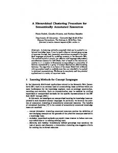
which when we combine with Equation (4), we arrive at Lemma 1. Simply put, when the spectra distribution satisfies Equation (5), then S shows a good clustering, i.e., the intra-similarity approaches 1, and the inter-similarity approaches 0. As an example, suppose we have a collection with 3 clusters as depicted in Table 1. The 3 topics are setup to be conceptually disjoint, and the similarity measure as well as the feature set are selected such that the outcome produces 3 distinct clusters. In this ideal condition, the spectra distribution (as shown in Figure 1) behaves as per Equation (5). Of course, real-world data sets that exhibit perfect clustering are extremely rare. This is especially the case for text collections, where its dimensionality is large but the data itself is sparse. In this case, most similarity measures do not rate two documents as distinctively similar, or different. If we perform a spectral analysis on the collection, we will end up with a spectra of G(S) that is very different from our example in Figure 1. As we will see next, this spectra distribution is much more complex. 3.2
Spectra Distribution in Large Data Sets
Point (iii) of Theorem 1 offers a strong conclusion between G(S) and its subgraphs. However, real-world data sets often exhibit a different characteristic. If we examine their corresponding G(S), we will see that the connections between G(S) and its subgraphs are weak, i.e., Lemma 1 no longer holds. Fortunately, we can still judge the cluster quality and estimate the number of natural clusters with spectral analysis. In this section, we present the proofs that
1 2 3 4 5 6
7 8 9 10 11 12
c1 c2 c3 c4 c5 m1 m2 m3 m4 d1 d2 d3
G(S) G(S11 ) G(S22 ) G(S22 (1)) G(S22 (2))
λ1 1 1 1 1 1
λ2 0.92 0.25 0.91 0.04 —
λ3 0.88 — 0.07 — —
λ4 0.25 — — — —
S11
λ5 0.06 — — — —
S22(1) S22 S22(2)
(a)
(b)
Fig. 1. The spectra distribution of the collection in Table 1: (a) Spectrum (> 0) of G(S) and its subgraphs; (b) a graphical representation of S. Note that all grey images in this paper are not “plots” of the spectra. Rather, they are a graphical way of summarizing the results of clustering for comparison/discussion purposes.
leads to the conclusion about cluster quality and k. But first, we need introduce the Cheeger constant. Let SV ⊂ V of G(S). We define the volume of SV as: vol(SV ) =
X
dv
(10)
v∈SV
where dv is the sum of all weighted edges containing vertex v. Further, let E(δSV ) be the set of edges, where each edge has one of its vertices in SV but not the other, i.e., SV . Then, its volume is given by: |E(δSV )| =
X
weight(vi , vj )
(11)
vi ∈SV ,vj ∈SV /
and by Equations (10) and (11), we derive the Cheeger constant: h(G) = min
SV ⊂V
|E(δSV )| min(vol(SV ), vol(SV ))
(12)
which measures the optimality of the bipartition in a graph. The magnitude |E(δSV )| measures the connectivity between SV and SV while vol(SV ) measures the density of SV against V . Since SV enumerates all subsets of V , h(G) is a good measure that finds the best bipartition, i.e., hSV, SV i. Perhaps, more interesting is the observation that no other bipartition gives a better clustering than the bipartition determined by h(G). Therefore, h(G) can be used as an indicator of cluster quality, i.e., the lower its value, the better the clustering.
Theorem 2. Given the spectra of G(S) as 1 = λ1 > λ2 > · · · > λn , if λ2 → 1, then there exists a good bipartition for G(S), i.e., a good cluster quality. p 2) Proof. From [9], we have the Cheeger inequality: (1−λ 6 h(G) < 2(1 − λ2 ) 2 that gives the bound of h(G). By this inequality, if λ2 → 1, then h(G) → 0. And since h(G) → 0 implies a good clustering, we have the above. For a given similarity measure, Theorem 2 allows us to get a “feel” of the clustering quality without actually running the clustering algorithm. This saves computing resources and reduces the amount of time the user waits to get a response. By minimizing this “waiting time” during initial analysis, we promote interactivity between the user and the clustering algorithm. In such a system, Theorem 2 can also be used to help judge the suitability of each supported similarity measure. Once the measure is decided, the theorem to be presented next, provides the user a starting value of k. Theorem 3. Given the spectra of G(S) as 1 = λ1 > λ2 > · · · > λn , ∃k > 2 such that αi → 1 and αi − αi+1 > δ (0 < δ < 1) for the sequence αi = λλ2i , (i > 2), where δ is a predefined threshold to measure the first large gap between αi ; and k is the natural number of clusters in the data set. Proof. Since Theorem 2 applies to both G(S) and its subgraphs G(Sii ), then we can estimate the cluster quality of the bipartition in G(Sii ) (as well as its subgraphs). Combine with Point (iii) of Theorem 1, we can conclude that the number of eigenvalues in G(S) (that approach 1 and have large eigengaps) give the value of k, i.e., the number of clusters. To cite an example for the above, we revisit Table 1 and Figure 1. By the Cheeger constant of G(S), SV = {c1 , c2 , c3 , c4 , c5 } and SV = {m1 , m2 , m3 , m4 , d1 , d2 , d3 } produces the best bipartition. Thus, S11 represents the intersimilarities in SV and S22 represents inter-similarities in SV . From Theorem 2, we can assess the cluster quality of G(S)’s bipartition by λ2 . Also, we can recursively consider the bipartitions of the bipartitions of G(S), i.e., G(S11 ) and G(S22 ). Again, the Cheeger constant of G(S22 ) shows that G(S22 (1)) and G(S22 (2)) are the best bipartition in the subgraph G(S22 ). Likewise, the λ2 of G(S11 ), G(S22 ), G(S22 (1)), and G(S22 ) all satisfy this observation. In fact, this recursive bisection of G(S) is a form of clustering using the Cheeger constant – the spectra of G(S22 ) contains the eigenvalues of G(S22 (1)) and G(S22 (2)), and G(S) contains the eigenvalues of G(S11 ) and G(S22 ) respectively (despite with some small “fluctuations”). As shown in Figure 1(a), λ2 of G(S) gives the cluster quality of the bipartition G(S11 ) and G(S22 ) in G(S); and λ3 of G(S), which corresponds to λ2 of G(S22 ), gives the cluster quality indicator for the bipartition G(S22 (1)) and G(S22 (2)) in G(S22 ), and so on. Therefore, if there exist k distinct and dense diagonal squares (i.e., Sii where 1 6 i 6 k) in the matrix, then λi of G(S) will be the cluster quality indicator for the i-th bipartition (2 6 i 6 k), and the largest k eigenvalues of G(S) give the estimated number of clusters in the data.
Table 2. The text collections used in our experiments to estimate k: we selected 4 classes of classic with each class containing 1,000 documents; 5 newsgroups with each newsgroup containing 500 documents; 2 categories of the webset with each category containing 600 documents. Collections Source # Classes # Documents classic ADI/CACM/CISI/CRAN/MED 5 5559 newsgroup UseNet news postings 17 7473 webset Categories in Yahoo [12] 10 6607
4
A Motivating Example
In this section, we discuss an example of how the theoretical observations discussed earlier work to close the gap between the algorithm and the user. For illustration, we assume that the user is given some unknown collection. If the user does not have pre-existing knowledge of the data, there is a likelihood of not knowing where to start. In particular, all clustering algorithms directly or indirectly require the parameter k. Without spectral analysis, the user is either left guessing what value of k to start with; or expend time and effort to find k using one of the existing estimation algorithm. In the case of the latter, the user has to be careful in setting kmax (see Section 5.2) – if it’s set too high, the estimation algorithm takes a long time to complete; if it’s set too low, the user risks missing the actual value of k. In contrast, our proposal allows the user to obtain an accurate value of k without setting kmax . Performance wise, this process is almost instantaneous in comparison to other methods that require a clustering algorithm. We believe this is important if the user’s role is to analyze the data instead of waiting for the algorithms. Once an initial value of k is known, the user can commence clustering. Unfortunately, this isn’t the end of cluster analysis. Upon obtaining the outcome, the user usually faces another question: what is the quality of this clustering? In our opinion, there is no knowledge discovery when there is no means to judge the outcome. As a result, it is also at this stage where interactivity becomes important. On this issue, some works propose the use of constraints. However, it is difficult to formulate an effective constraint if the answer to the above is unknown. This is where spectral analysis plays a part. By Theorem 2, the user is given feedback about the cluster quality. At the same time, grey images (e.g., Figure 1(b)) can also be constructed to help the user gauge the outcome. Depending on the feedback, the user may then wish to adjust k, or use another similarity measure. In either case, the user is likely to make a better decision with this assistance. Once the new parameters are decided, another run of the clustering algorithm begins. Our proposal would then kick in at the end of each run to provide the feedback to the user via Theorem 2. This interaction exists because different clustering objectives can be formulated on the same data set. At some point, the user may group overlapping concepts in one class. Other
0.8
0.5
0.5
0.4
0.4
0.5 0.4 0.3
eigenvalue
0.6
eigenvalue
eigenvalue
0.7
0.3
0.3
0.2
0.2
0.2 0.1 2
4
6
8
10 12 14 16 18 20
index of eigenvalue (λ −−λ ) 2
20
(a) web2
0.1
2
4
6
8
10 12 14 16 18 20
index of eigenvalue (λ −−λ ) 2
(b) clasic4
20
0.1 2
4
6
8
10 12 14 16 18 20
index of eigenvalue (λ −−λ ) 2
20
(c) news5
Fig. 2. The spectrum graphs and the graphical representation of their clustering for all 3 collections: the first two data sets are conceptually disjoint, and the last has overlapping concepts.
times, the user may prefer to separate them. In this aspect, our approach is non-intrusive and works in tandem with the user’s intentions.
5
Empirical Results
The objective of our experiment is to provide empirical evidence on the viability of our proposal. In particular, we show that our approach accurately estimates the correct number of clusters. Due to space constraints, we shall limit our discussion to only one set of experiment. Readers interested in the results of other data sets can refer to Appendix A. The details of the 3 text collections used in our experiment is given in Table 2. 5.1
Estimating the Number of Clusters
In practice, we can estimate k by using Theorem 3. However, for the purpose of illustration, we will walkthrough the analysis. Since λ1 is always 1, our analysis begins from λ2 . In Figure 2, we have marked out the large eigenvalues whose gap is larger than the rest. This gap can be best identified by the big stair steps among the eigenvalues. According to Theorem 3, the number of such eigenvalues (including λ1 ) gives the number of clusters. We can verify this by analyzing their corresponding grey images in the same figure. Figure 2(a) shows the web2 collection with just 2 class labels and their topic being completely disjoint: finance and sport. In this case, notice that λ2 has a
Table 3. Comparison with 3 well-known indexes: the Calinski and Harabasz (CH) index; Krzanowski and Lai (KL) index; and Hartigan (Hart) index with 3 well-known √ clustering algorithms: bisecting k-means, graph-based, and hierarchical – a ( ) indicates a correct estimation. Bisecting k-means Graph-based Hierarchical web2 classic4 news5 web2 classic4 news5 web2 classic4 news5 √ CH 5 2 3 3 3 3 7 2 5( ) KL 29 17 22 27 21 22 22 21 9 √ √ Hart 6 13 4( ) 6 10 4( ) 1 2 1
higher value than the others. Since the remaining eigenvalues fall along a smooth curve, this phenomenon conforms to Theorem 2 and 3. In this case, we therefore conclude k = 2. At the same time, the high value of λ2 indicates that this is a good clustering by the similarity measure used. In the second case, classic4 has 4 topics from scientific abstract from different research domains: computing algorithms, information retrieval, aerodynamics and medicine. They are conceptually disjoint, which can be observed from Figure 2(b) where there are 4 distinctive diagonal squares. From its spectra graph, we observe that λ2 , λ3 and λ4 show higher values and wider gaps than other eigenvalues. Again by the same theorem, our method obtains the correct number of clusters, i.e., k = 4. The third collection is the most challenging. There are 5 topics: atheism, comp.sys, comp.windows, misc.forsale and rec.sport. Unlike the previous two collections, the topics are not disjoint. In this case, both comp.sys and comp.windows belong to the broader topic of comp in the newsgroup. Therefore, the graphical representation in Figure 2(c) do not show a set of distinctive squares along its diagonal. When we apply our analysis, only λ2 , λ3 , and λ4 have a higher value and a wider gap than the others. So by our theorems, k = 4. This conclusion is actually reasonable since comp is more different from the other topics. If we observe the grey image in Figure 2(c), we see that the second and third squares appear to “meshed” together – an indication of similarity between comp.sys and comp.windows. Furthermore, comp.sys, comp.windows and misc.forsale can also be viewed as one topic. This is because misc.forsale has many postings on buying and selling of computer parts. Again, this can be observed in the grey image. On the spectra graph, λ4 is much lower than λ2 , λ3 , and closer to the remaining eigenvalues. Therefore, λ4 may not be counted as the number of clusters. Thus, it is possible to conclude k = 3 by Theorem 3. Strictly speaking, this is also an acceptable estimation. Thus, the onus is on the user to judge the actual value of k, which is really problem-specific as illustrated in the Section 4. We end this section by discussing the performance of our method. In text collections, the data is often sparse, i.e., the number of non-zero entries h in S is less than the number of zero entries. Therefore, the complexity of transforming S to L is O(h). To compute the eigenvalues, we used the Lanczos method which
is capable of obtaining the eigenvalues in k ≪ n iterations (converges very quickly) [10]. Since the complexity of each iteration is O(h+n), the complexity of our method is O(k(h+n)). If we ignore the very small k in real computations, the complexity of our method becomes O(h + n). There are fast Lanczos packages (e.g., LANSO [13], PLANSO [14]) for such computation. 5.2
Comparison with Existing Methods
There are many methods to estimate the number of clusters in a data set. To date, most require choosing an appropriate clustering algorithm, e.g., kmeans, where it is ran multiple times with predefined cluster numbers from 2 to kmax . The optimum k is then obtained by an internal indexed based on the clustering outcome. The key difference between these methods is in the index used. In this experiment, we compared our results to 3 widely used statistical methods [15] on 3 well-known clustering algorithms (see Table 3). From the table, we found that all 3 indexes managed to get only 1 out of the 3 estimations right. Although the Hart index correctly estimated 4 clusters in news5, it fails to handle the conceptually disjoint web2 and classic4. Worse, most of the estimation are way off-track. For example, the KL index predicted k = 29 on web2! Furthermore, to the best of our knowledge, many of these methods report results on data sets with low dimensionality. Hence, our experiment reveals how sensitive these indexes are to the choice of clustering algorithms and the dimensionality of the data set. In contrast, our proposal is independent of any clustering algorithm, is wellsuited to high dimensional data sets, has low complexity, and can be easily implemented with existing packages. Clearly, our proposal remarkably outperforms all 3 methods in terms of speed and accuracy.
6
Related Works
Underlined by the fact that there is no clear definition of what is a good clustering [2, 16], the problem of estimating the number of clusters in a data set is arguably a difficult one. Over the years, several approaches to this problem have been suggested. Among them, the more well-known ones include crossvalidation [17], penalized likelihood estimation [18, 19], resampling [20], and finding the ‘knee’ of an error curve [2, 21]. The problem with these techniques is that they either make a strong parametric assumption, or they are computationally expensive. For example, both cross-validation and penalized likelihood estimation require some form of input parameters, e.g., the number of cross validations or the MML. On the other hand, techniques such as resampling and finding the ‘knee’ of an error curve are examples of CPU-intensive methods. In resampling, the natural number of clusters are discovered by repeated clustering of samples drawn from the original data set; while in the case of finding the ‘knee’ of an error curve, each potential value of k requires a run of the clustering algorithm.
Unfortunately, these methods become undesirable when the objective of estimating k is to facilitate productive cluster analysis. What is really needed is a “roadmap” containing the necessary information for the user to perform the knowledge discovery. In our case, this “roadmap” is the result of analyzing the spectra of the text collection. More importantly, this result is easy to obtain, i.e., no parameters needed1 nor computationally intensive. Furthermore, the spectra contains other information besides k – it also provides a means to estimate the cluster quality of the data set in question. Spectral analysis has a long history of wide applications in the scientific domain. Usually, the data under study is represented in a matrix, where the eigenvectors or eigenvalues are derived to understand certain properties of the data. In the database community, eigenvectors have applications in areas such as information retrieval (e.g., singular value decomposition [22, 23]), collaborative filtering (e.g., reconstruction of missing data items [24]), and Web searching [25]. Meanwhile, eigenvalues are used in analyzing graphs that are abstraction of real world objects and their relationships. Application examples include the understanding of communication networks [9] and Internet topologies [26]. The application of spectral analysis in data mining only became popular in the recent years [27]. To the best of our knowledge, we have yet to come across works that use eigenvalues to assist cluster analysis. Most proposals that use spectral techniques for clustering focused on the use of eigenvectors, not eigenvalues. And for those that use eigenvalues, their applications are limited to graph-based data sets (e.g., network topologies), not text collections. Our work is therefore novel in two ways: we present an efficient and effective solution to close the gap between the clustering algorithms and the user; and we apply the results of eigenvalue analysis to text collections.
7
Conclusions
In this paper, we demonstrate a concrete case of our argument on the need to close the gap between data mining algorithms and the user. We exemplified our argument by studying a well-known problem in clustering that every user faces when starting the analysis: “What value of k should we select so that the analysis converges quickly to the desired outcome?”. We answered this question, in the context of text collections, with spectral analysis. We show (both argumentatively and empirically) that if we are able to provide a good guess to the value of k, then we have a good starting point for analysis. Once the “ground” is known, data mining can proceed by changing the value of k incrementally from the starting point. This is often better than the trial and error approach. In addition, we also show that our proposal can be used to estimate the quality of clustering. This process, as part of cluster analysis, is equally important to the success of knowledge discovery. Our proposal contributes in part to this insight. 1
From the user’s perspective, δ is unknown.
In the general context, the results shown here also demonstrate the feasibility to study techniques that bridge the algorithms and the user. We believe that this endeavor will play a pivotal role to the advancement of knowledge discovery. In particular, as data takes a paradigm shift into continuous and unbounded form, the user will no longer be able to devote time in tuning parameters. Rather, their time should be spent on interacting with the algorithms, such as what we have demonstrated in this paper.
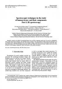
Appendix A We have also conducted experiments to verify our proposal on real-life gene expression data sets. The first data set is obtained from a study of gene expression in the budding yeast Saccharomyces cerevisiae; and the second data set is obtained from a study of 60 cancer cell lines derived from tumours of a variety of tissues and organs. Saccharomyces cerevisiae This data set comes from a study of gene expression in the budding yeast Saccharomyces cerevisiae during the diauxic shift [28], with each gene having 79 arrays. Each cell in the gene expression matrix represents the measured Cy5/Cy3 fluorescence ratio at the corresponding target element on the appropriate array. For our experiment, we selected four clusters (64 genes in total) [28] who share similar expression patterns and are annotated along the same biological pathway. They are protein degradation (cluster C), chromatin structure (cluster H), protein synthesis (cluster F), and glycolysis (cluster E). For simplicity of experimental setup but without loss of accuracy, we do not impute the cells using complex and CPU-intensive techniques. Instead, we simply filled the cells without data in the gene expression matrix with zeros. On top of that, we used the Pearson correlation coefficient as the measure of similarity, where its range is within [−1, 1]. To get the similarity values to within the range of [0, 1], we apply the translation operator to each similarity value before halving them. From these preprocessing, we obtain the similarity matrix and its corresponding spectra as shown in Figure 7(a). By Theorem 3, the spectra graph suggests k = 4 in this particular data set, which corresponds to our experimental setup. At the same time, the grey scale plot in Figure 7(b) provides suggestion that it is also possible to set k = 2, i.e., to partition the data set into 2 clusters. In this case, protein synthesis and glycolysis would be grouped, since they have a higher similarity than protein degradation and chromatin structure. NCI 60 The cDNA microarrays were used to examine the variation in gene expression among the 64 cell lines from the National Cancer Institute’s (NCI) anti-cancer
0.35 0.3
eigenvalue
0.25 0.2
(1)
0.15
(2)
0.1 0.05 0 −0.05
(3) 2
10
20
30
40
index of eigenvalue (λ2−−λ64)
50
60
64
(4)
Fig. 3. The Saccharomyces cerevisiae gene expression data set: (a) its spectrum graph; and (b) the grey scale plot where (1) is protein degradation, (2) is chromatin structure, (3) is protein synthesis and (4) is glycolysis.
drug screen [29]. Again, we selected a subset of 1,161 cDNAs measured across 64 cell lines, which was described and used in [29] and shown in Figure 7. The corresponding data set can be downloaded from http://genome-www.stanford.edu/ sutech/download/nci60/dross clusters.tgz. We used similar preprocessing techniques as per our experiment above. The spectrum of this data set is shown in Figure 7(a), and clearly indicates the presence of four clusters. This estimation was confirmed to be correct by the plot obtained from the given URL, which we have replicated in Figure 7(b) and discussed in the original paper.
References 1. Salvador, S., Chan, P.: Determining the number of clusters/segments in hierarchical clustering/segmentation algorithms. Technical report 2003-18, Florida Institute of Technology (2003) 2. Tibshirani, R., Walther, G., Hastie, T.: Estimating the number of clusters in a dataset via the gap statistic. Technical Report 208, Dept. of Statistics, Stanford University (2000) 3. Sugar, C., James, G.: Finding the number of clusters in a data set : An information theoretic approach. Journal of the American Statistical Association 98 (2003) 4. Dempster, A., Laird, N., Rubin, D.: Maximum likelihood from incomplete data via the em algorithm. Journal of Royal Statistical Society 39 (1977) 1–38 5. Evans, F., Alder, M., deSilva, C.: Determining the number of clusters in a mixture by iterative model space refinement with application to free-swimming fish detection. In: Proc. of Digital Imaging Computing: Techniques and Applications, Sydney, Australia (2003) 6. Yang, Y., Guan, X., You, J.: CLOPE: A fast and effective clustering algorithm for transactional data. In: Proc. of KDD, Edmonton, Canada (2002) 682–687 7. Strehl, A., Ghosh, J., Mooney, R.: Impact of similarity measures on web-page clustering. In: Proc. of AAAI Workshop on AI for Web Search. (2000) 58–64
0.1
eigenvalue
0.08 0.06 0.04 0.02 0 −0.02
2
10
20
30
40
50
60
70
index of eigenvalue (λ −−λ ) 2
(a)
70
(b)
Fig. 4. The NCI60 gene expression data set: (a) the grey scale plot at http://genomewww.stanford.edu/nci60/figures.shtml; and (b) its spectrum graph.
8. Jain, A.K., Murty, M.N., Flynn, P.J.: Data clustering: A review. ACM Computing Surveys 31 (1999) 264–323 9. Chung, F.R.K.: Spectral Graph Theory. Number 92 in CBMS Regional Conference Series in Mathematics. American Mathematical Society (1997) 10. Golub, G., Loan, C.V.: Matrix Computations (Johns Hopkins Series in the Mathematical Sciences). 3rd edn. The Johns Hopkins University Press (1996) 11. Landauer, T., Foltz, P., Laham, D.: Introduction to latent semantic analysis. Discourse Processes 25 (1998) 259–284 12. Sinka, M.P., Corne, D.W.: A Large Benchmark Dataset for Web Document Clustering. In: Soft Computing Systems: Design, Management and Applications. IOS Press (2002) 881–890 13. LANSO: (Dept. of Computer Science and the Industrial Liason Office, Univ. of Calif., Berkeley) 14. Wu, K., Simon, H.: A parallel lanczos method for symmetric generalized eigenvalue problems. Technical Report 41284, LBNL (1997) 15. Gordon, A.: Classification. 2nd edn. Chapman and Hall/CRC (1999) 16. Kannan, R., Vetta, A.: On clusterings: good, bad and spectral. In: Proc. of FOCS, Redondo Beach (2000) 367–377 17. Smyth, P.: Clustering using monte carlo cross-validation. In: Proc. of KDD, Portland, Oregon, USA (1996) 126–133 18. Baxter, R., Oliver, J.: The kindest cut: minimum message length segmentation. In: Proc. Int. Workshop on Algorithmic Learning Theory. (1996) 83–90 19. Hansen, M., Yu, B.: Model selection and the principle of minimum description length. Journal of the American Statistical Association 96 (2001) 746–774
20. Roth, V., Lange, T., Braun, M., Buhmann, J.: A resampling approach to cluster validation. In: Proc. of COMPSTAT, Berlin, Germany (2002) 21. Tibshirani, R., Walther, G., Botstein, D., Brown, P.: Cluster validation by prediction strength. Technical report, Stanford University (2001) 22. Deerwester, S., Dumais, S., Landauer, T., Furnas, G., Harshman, R.: Indexing by latent semantic analysis. JASIS 41 (1990) 391–407 23. Husbands, P., Simon, H., Ding, C.: On the use of singular value decomposition for text retrieval. In: Proc. of SIAM Comp. Info. Retrieval Workshop. (2000) 24. Azar, Y., Fiat, A., Karlin, A., McSherry, F., Saia, J.: Spectral analysis of data. In: ACM Symposium on Theory of Computing, Greece (2001) 619–626 25. Kleinberg, J.M.: Authoritative sources in a hyperlinked environment. Journal of the ACM 46 (1999) 604–632 26. Vukadinovic, D., Huan, P., Erlebach, T.: A spectral analysis of the internet topology. Technical Report 118, ETH TIK-NR (2001) 27. Azar, Y., Fiat, A., Karlin, A., McSherry, F., Saia, J.: Spectral analysis of data. In: Proc. of STOC, Crete, Greece (2001) 619–626 28. Eisen, M.B., Spellman, P.T., Brown, P.O., Botstein, D.: Cluster analysis and display of genome-wide expression patterns. Proc. Natl. Acad. Sci. USA 95 (1998) 14863–14868 29. Ross, D.T., Scherf, U., Eisen, M.B., Perou, C.M., Rees, C., Spellman, P., Iyer, V., Jeffrey, S.S., de Rijn, M.V., Waltham, M., Pergamenschikov, A., Lee, J.C., Lashkari, D., Shalon, D., Myers, T.G., Weinstein, J.N., Botstein, D., Brown, P.O.: Systematic variation in gene expression patterns in human cancer cell lines. Nature 24 (2000) 227–235