Effective Subspace Clustering with Dimension ... - Semantic Scholar

Effective Subspace Clustering with Dimension Pairing in the Presence of High Levels of Noise Andrew Foss and Osmar R. Zaïane University of Alberta, Canada {foss, zaiane}@cs.ualberta.ca From both these challenges, we can see that there is a compelling motivation for inspecting subspaces. Firstly, it is unlikely that meaningful clusters exist in the fulldimensional space. Secondly, if we fail to inspect the subspaces we may miss clusters. We also see that attempting to cluster accurately in high-dimensionality is very inefficient while clustering subspaces faces two challenges, first we have to find the interesting subspaces and, if they are large we still have an efficiency or accuracy problem. Secondly, the number of possible subspaces is exponential in the dimensionality. There are two distinct problems, determining the subspaces and then clustering them. We show that it is possible to do both without clustering more than a twodimensional space. 2D clustering or spatial clustering is a well-studied problem and we earlier presented a parameter-free algorithm TURN* that performed as well or better than other well-known methods [22]. This algorithm can be used in the method presented in this paper or indeed any 2D algorithm but we found that we got excellent results with a very simple approach taking advantage of the positive side of higher dimensionality. As our results show, while higher dimensionality means greater sparsity, this also means that false positives are strongly suppressed while the false negative rate can be estimated allowing many to be recovered. While TURN* and virtually all subspace algorithms involve a series of iterations, our new method involves a single computation making it very fast as well as the added advantage of being deterministic. In the next section we present motivating related work. The following section provides definitions and then the methodology of the new algorithm, MAXCLUS is presented. After that we present the results and then conclude and discuss extensions we are pursuing.

Abstract Attempts at clustering large and high dimensional data have been made with a focus on scalability. While still inefficient for more complex problems, the effectiveness is also questionable because data becomes very sparse in a high dimensional space. If clusters exist in the data, they tend to remain hidden in some unidentified sub-spaces. So far, the few solutions to this problem have not been able to handle high levels of noise and are often inefficient. Most clustering solutions also require fine-tuning of parameter settings, which are difficult or impossible to set in advance especially by a novice user. We propose a new method, MAXCLUS, which first identifies sub-spaces where clusters could be located then pinpoints the clusters in each sub-space. MAXCLUS has proved robust even with high levels of noise and is very efficient and accurate with little or no parameter adjustment on a wide range of problems outperforming existing approaches.

1. Introduction The ‘curse of dimensionality’ coined by Richard Bellman [6] is that as the dimensionality increases the data typically becomes increasingly sparse so that it becomes increasingly difficult to use the distances between data points to identify clusters and outliers. Literally, every point becomes an outlier [7]. This problem becomes acute when any type of approximation is used for determining the neighbourhood of a data point. Houle and Sakuma [27] have given a fast approximate similarity search algorithm (SASH) suited to very high-dimensional datasets. They compare their method to sample sequential search and other methods. Their results show that efficiency can only be improved if a level of error is accepted. Computing exactly the matrix of similarity is quadratic in the number of points, so, in any large dataset, all current methods fall back on some type of approximation. Another problem is that full-dimensional clustering can miss clusters that only exist in some subspace. Parsons et al. [38] demonstrate on a simple dataset how clustering in just 3D using k-means misses clusters generated in 2D.

2. Motivating related work A useful review of subspace clustering has been given by Parsons et al. [38]. As they discuss, there are two principal techniques applied to this problem. The first is feature transformation and the second feature selection. In feature transformation linear combinations of the features (dimensions) are formed using techniques such as Principal Component Analysis (PCA), Singular Value

1

out that while random projection has promising theoretical properties it results in highly unstable clustering performance. They attempt to resolve this using a cluster ensemble approach. That is, they perform a series of random projections into a lower dimensional space followed by clustering and then combine the results. Random projection involves projecting the full space using a randomly generated transformation matrix. While this may reveal that a set of points are clustered together, the subspace in which this cluster actually exists is not known. This makes the results difficult to interpret.

Decomposition (SVD) and Random Projection [20]. This works well in certain circumstances but also faces certain problems. These techniques usually require the computation of a covariance matrix, which is expensive, and retain all the features. The later means that subspace clusters can still be obscured by redundant features and the final result is more difficult to interpret. Clustering algorithms incorporating this approach include the work of Ding et al. [16], Hinneburg and Keim [28], and Fern and Brodley [20].

2.1 Feature Selection 2.2 Subspace Search Feature selection involves searching for feature subsets that meet some criterion. Commonly a greedy sequential search is performed through the feature space (e.g. [31, 40, 47]). Exhaustive search is intractable so some heuristic has to be employed to constrain the search space. Approaches generally fall into two categories, wrapper and filter methods. The wrapper methods use the mining algorithm iteratively adjusting weights on the dimensions to optimise the output. Filter approaches use some method to select features. Dash et al. [15] use entropy and make the point that using wrapper approaches leaves the process dependent on the parameter settings on which almost all clustering algorithms depend. At the same time they require a measure of goodness of clustering about which there is no general agreement in the unsupervised case. Their filter approach is based on the idea that spaces with clusters have lower entropy than those where the points are more evenly spread. They define entropy in terms of point to point distances, dense regions having many examples of low distances. All those doing filtering of features in an unsupervised way have to get some measure of the likelihood of clusters existing in the subspace. Trying to estimate clustering without clustering as done, for example, by Dash et al. is certainly more approximate than an actual clustering and could be confounded by, for example, many small noise clusters. Their method involves many heuristics and parameters and they try to avoid the quadratic of distance computation by using a grid but this faces even more severe computational costs in high dimensionality. This illustrates that any method that attempts to handle the full dimensional space in order to locate the subspaces, as many authors do, runs into great difficulties unless the dataset is especially suited to the method. Kim et al. [29] discuss the fact that many different criteria can exist as to the goodness of clustering in a subspace and propose a method that employs the Pareto front, in effect a voting scheme among the various criteria. They approach the search problem using an Evolutionary Local Selection Algorithm (ELSA). Others have taken to random searching [1, 9, 20]. Fern and Brodley [20] point

Subspace search methods can be divided into ‘top down’ and ‘bottom up’. Top down methods operate on the whole space iteratively adjusting weights on the dimensions based on the results of each stage until the results stabilise. Bottom up methods build subspaces starting with assessment of single dimensions. Typically dense units are sorted in each dimension and their projections into two and higher dimensions are collected. This is the method adopted by CLIQUE, the first of this type of algorithm [2]. CLIQUE scans the dataset once building the dense units in each dimension. Then it combines the projections and checks them against the database to ensure they are also dense building larger and larger subspaces. As CLIQUE exhaustively searches, the cost increases exponentially with the size of the subspaces searched. CLIQUE then computes minimal cluster descriptions by first greedily covering the region by a number of maximal rectangles and then discarding the redundant rectangles to create a minimal cover. This is then output as a DNF description. While CLIQUE outputs descriptions of dense regions, no attempt is made to distinguish subspaces containing specific sets of points or the clustered points themselves. ENCLUS [12] is a version of CLIQUE that uses an entropy measure rather than simple bin density. ENCLUS adds to CLIQUE by evaluating the clustering, not only on the coverage - the proportion of the data contained in the cluster - but also the density. They also seek that dimensions should be somewhat correlated. CLIQUE and ENCLUS use a fixed grid size while the other group of bottom-up methods adapt the grid to the data. For example, a high frequency grid can be imposed and then adjacent bins with similar densities above the threshold are merged as is performed in the MAFIA algorithm [25]. Otherwise it is much like CLIQUE. Other adaptive grid algorithms are CBF [13], CLTree [33] and DOC [39]. CBF is faster than CLIQUE but at a small cost in precision. CLTree [33] uses a decision tree approach comparing relative emptiness with fullness and an information gain criteria to repeatedly partition the space 2

perform subspace identification in document clustering via an iterative alternating optimization process. Another approach is to set weights on each dimension. COSA [21] is an offering from the statistical community. which uses iterative runs of any clustering algorithm to adjust the weights with a penalty based on the negative entropy of the weight distribution. Domeniconi et al. [17] introduce a Locally Adaptive Clustering algorithm (LAC) which starts from a set of k centroids and a set of weights and adapts the weights to approximate a group of k Gaussians from the dataset while Candillier et al. [14] use a maximum likelihood estimation approach (SSC) to approximate the data as a set of k Gaussians. An example of using an objective function is Tseng and Kao [42] who employed a simplified Hubert’s Γ statistic to validate the clustering. Yip et al. developed HARP [45] and then SSPC [46]. HARP is a hierarchical clustering method. Starting with N clusters the internal merging thresholds are progressively loosened until the desired k clusters is achieved. While intended to resolve the problem of mandatory parameters it still requires two and is very slow due to the hierarchical approach. SSPC is based on k-medoids and benefits when some training data is available but can cluster without training data. Our results show it to be the best of those studied but, without some labelled data, only some runs find the correct solution due to the random start. It also needs to know k and certain other parameters. Linear scaling is claimed but the speed is still too low for larger datasets.

into hyper-rectangular areas. Typically for a decision tree this approach tends to go too far and needs pruning. The authors give an example of a space containing two clusters that is partitioned into 14 areas. PROCLUS [3] was the first of its type. It uses the kmedoids technique as in the clustering algorithm CLARANS [36] and uses a locality analysis to find the set of dimensions associated with each cluster. It requires k, the number of clusters and l, the average dimensionality of the subspaces. A random set of k well separated medoids is selected and a set of dimensions is chosen for each medoid based on the points closest to it and the dimensions on which these are most close. Points are then assigned to their nearest medoid based on the chosen set of dimensions and Manhattan segmental distances. The total number of dimensions is limited to k.l. The clustering is evaluated, highly disperse medoids replaced and the process iterates. The method tends to find hyper-spherical clusters and similar sized subspaces and is sensitive to the parameter settings. PROCLUS uses sampling which improves speed at the risk of missing some clusters. ORCLUS [4] extended PROCLUS to seek non-axis parallel subspaces but the running time is cubic in the dimensionality. FINDIT [43] is short for a Fast and Intelligent subspace clustering algorithm using Dimension voting. The key idea is that closeness in many dimensions is more important than being very close on a few. FINDIT uses a medoid approach and sampling for better speed. Parsons et al. [38] compared MAFIA [25] and FINDIT on two datasets. The first had n = 100,000 and d = 20 and the second was the same size but with d = 100. On the first, FINDIT completed the task accurately while MAFIA found the clusters but missed some dimensions. One the second FINDIT missed many dimensions and an entire cluster while MAFIA missed one dimension in several clusters and split one cluster into three. This behaviour of MAFIA is a result of the pruning process. The running time of MAFIA was much superior to FINDIT until the dataset sized reached 4 million where the advantage of its sampling process started to give it an increasing edge. δ-clusters [50] brought out the concept of coherent clusters. It captures the coherence exhibited by a subset of objects on a subset of attributes while allowing for missing values. They present the FLOC algorithm and claim it efficiently produces near-optimal clustering. This approach is motivated especially by bioinformatics where finding related genes, say, means seeing similar response patterns even if the absolute response values differ. They claim that the biclustering approach of Cheng and Church [11] is a special case of their δ-clusters. The method starts from k seeds and is quadratic in N and D. Other developments on the idea of biclustering are [51] and Melkman and Shaham [34] who use a randomised approach to avoid an exhaustive search. Li et al. [32]

2.3 Conclusion As we see there are a few generic methods presented in various skilful ways but each with obvious drawbacks. Hierarchical algorithms are very slow and require key parameters. Projected clustering is often faster but suffers from the exponential cost of searching all possible projected subspaces, the answer is pruning but this can cost accuracy. k-medoid approaches are very dependent on the initial seeds and also have key parameters. Like all methods that optimise an objective function there can be many iterations making the running time impractical for larger problems and the algorithm may stop in a local minimum. Algorithms with an objective function are also usually biased toward spherical clusters. If well-defined clusters exist in some subspaces, it should be possible to find them in an efficient, accurate and deterministic fashion. This is our motivation for this paper.

3. Preliminary definitions The words ‘attributes’ and ‘dimensions’ have the same meaning in this paper. Noise dimensions ND are those

3

every dimension by chance is small – we can reclaim tail points with little chance of noise contamination. Thus, if we want to maintain such a proportion α has to increase with subspace size. For example, α = 0.45 with a subspace of 9 has to rise to α = 0.65 with 18. Also increasing α with N maintains the true positive collection rate while slightly increasing the false positive rate (see table 1). In these experiments, we did not allow dense areas to overlap due to this ‘expansion’.

dimensions where no discernible clusters or dense areas can be detected after filtering the background noise. Clustered dimensions CD are dimensions that are not noise dimensions. A database DB is a set of N points each of maximum dimension D where the set of dimensions D = {ND, CD}. ND = |ND|, CD = |CD|. A clustering relationship between two dimensions exists where a set of points P ∈ DB have similar values to each other in each of the two dimensions such that such a similarity is unlikely to arise by chance alone. Bins B (B = |B|) are equiwidth segments of a dimension such that B = N / 15 (N ≥ 1500), B = 100 (1500 > N ≥ 300), B = N / 3 (N < 300). Thus the mean bin size m = N / B. A sequence of p above average density bins is flagged as a dense area when the accumulated total bin size T – m p > 2.5 m. Areas flagged as dense are expanded by a factor α p (see section 3.1). A maximal subspace S ∈ CD is a set of dimensions such that for all pairwise combinations of the members of S, a clustering relationship exists involving the same set of points P ∈ DB. Suppose the clustering relationship between any two members sa, sb in S ∈ CD (1 ≤ a, b ≤ |S|) consists of a set of clusters labelled {1, 2, … kab}. We call these the class numbers for the clustering relationship. Then the set of clusters C in S are sets of points P ∈ DB such that in each two dimensional clustering relationship between the members of S, all members of P have the same class number.

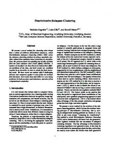
Figure 1: Clustering Relationship Graph example.

4. Methodology The difficult problems in the field of clustering lie in attempts to cluster above 10-15 dimensions [7] where it has been shown that any sub-quadratic method of neighbourhood determination shows an increasingly degraded level of accuracy [27] and even with a quadratic cost, the relative difference between the far and near neighbours of any object declines making clustering decisions moot. If clusters exist in subspaces, finding them through clustering on all dimensions is often likely to fail. In our previous work [22] we showed that a satisfactory clustering could be obtained in 2D even in the face of considerable structured noise without user adjustable parameters. If we restrict ourselves to twodimensional clustering, we can use these results to generate a graph based on the clustering relationships of pair-wise dimensions from which we can extract first the subspaces and then the clusters from them. Finding the subspaces is simply the problem of enumerating the maximal cliques in this graph, which we call the Clustering Relationship Graph (CRG). The graph vertices are the dimensions in the data, and the edges of the graph represent the existence of clusters in the 2 dimensional space formed by the two dimensions linked by the edge. Figure 1 illustrates an example with nine dimensions and three cliques, one with 5 vertices and two with 3, one overlapping the 5-clique sharing two dimensions.

3.1 Notes on parameters The constants that determine the bin size and the noise filter were set as they consistently allowed us to remove white noise over a wide range of N and D while detecting clustered areas generated by Gaussian distributions. To remove grey noise such as banding on images, the constant 2.5 could be increased. If the clusters are very small with high variance, then they may not be detected, however, this is a generic problem of determining whether a bin is dense by chance. Our 100% accuracy rate for collecting the attributes of subspaces on synthetic datasets started to degrade slightly with cluster standard deviations ≥ 3. The algorithm permits providing sample noise dimensions so that these constants can be automatically adjusted to suit the data set. With respect to parameter α, the probability of finding a fixed proportion of cluster members decreases with increasing number of attributes in a subspace as long as there is some stochasticity in the production of the members and hence the distribution has tails. At the same time, since for subspaces of size 3 and increasingly above this, noise is strongly suppressed by probability – the probability of a point falling in or near a dense area on

4

The clique enumeration problem is hard but research on random SAT problems has shown that almost all (random) graphs can be handled efficiently by an algorithm that prunes its branching effectively [e.g 19, 24]. Optimal partitioning of a graph [5], the Discrete Clustering Problem [18] or clustering of the elements of a dissimilarity matrix (the Bandwidth Minimisation problem [23]) are also in general hard problems, so efficient and accurate clustering is always dependent on the instance to be clustered not being inherently hard. For maximal clique enumeration we utilise a novel algorithm based on [8]. The details will be presented elsewhere but it is important to realize that the actual algorithm utilised is immaterial for the purpose of this paper because we are presenting a framework into which any effective clique enumeration algorithm can be plugged. If the cliques are all disjoint, then this algorithm is sub-quadratic in CD. Sparse data containing small cliques is handled most efficiently. This is often the case in large databases where sparsity is a natural consequence of high dimensionality. Clique enumeration is a very important element in studying gene expression [52]. This paper [52] argues for exact rather than approximate solutions and presents a general framework for handling even very high dimensional exponential problems using modern supercomputers. Those wishing to use our approach on highly complex problems can readily adopt such solutions.

density (see section 3). This works very well on real and synthetic data in distinguishing between real density and noise. Real data always has an element of stochasticity. This masks small effects and if we attempt to recover them, artifacts are inevitable. A threshold has to be set for filtering noise and we choose a constant multiple of the average bin density (see section 3). Distinguishing cluster peaks from noise is critical to the method. The method does algorithmically what an observer would do who visually inspects each dimension. The noise filtering parameters are set so the algorithm (typically) agrees with visual inspection. If no cluster is visible even on a single dimensional projection, it is much less likely to exist in higher dimensionality and thus how can we say it exists or expect any density-based algorithm to find it? Next all pairs of dimensions in CD are checked for clustering. If two dimensions have clustering, dense areas will occur in the intersection of at least one of their respective dense classes. If not then the points will be spread out across the range defined by the other dimension giving a much lower density. Just the dense intersections are inspected and a statistic is computed from the relative density observed based on the ratio of the density of intersecting bins and the mean bin density. This can be done in a single O(N) pass over the data. The statistics for the pairs are sorted. They either form into one or two classes. Either all the pairs have clustering – one class – or some do and some do not – two classes. In the latter case a simple bisection is done to separate the two class cases allowing the pairs with real clustering to be identified. From these results a graph is drawn with the attributes as nodes and the statistics as edge weights. After the bisection, only the edges indicating a clustering relationship are kept. Each edge contains not only the density statistic but also clustering information for every point, which we utilise to extract the clusters. Now we have a set of attribute relationships, which we can envision as a graph and we only need to enumerate the maximal cliques of the graph to output the subspaces. The final step is to recover the clusters from the cliques. This is also straightforward. We label each point involved in the clustering on all the edges of the clique by concatenating in sequence its class number on each edge (the number of the clustering on each 2D comparison). For example, suppose a subspace has 3 attributes representing 3 clustering relationships (edges). In two of these only one cluster exists but in the third there are two. Thus every point clustered in every 2D clustering represented by these edges has a label {111} or {112}. The third digit indicates the membership of the two clusters on the third edge. These concatenated labels are then sorted and the groups of identical labels are easily recovered. This produces the clusters that conform to our definitions given above.

4.1 The MAXCLUS algorithm Subspace clustering is essentially two problems. Finding the subspaces and enumerating the clusters. They can be done in either order; we choose to find the subspaces first. The method proceeds in several stages. 1. 2. 3. 4.

5.

Normalize data and hash into bins. Identify noise dimensions (ND) and dimensions containing clustering (CD). Find all pairs in CD with a clustering relationship. Present this result as a graph of the clustering relationships and enumerate the maximal subspaces based on the cliques in the graph. Extract the clusters for the subspaces based on the clustering relationship on each edge.

After pre-processing (stage 1) the individual dimensions are inspected for dense regions. Each distinct dense region is given a class number. Dimensions with no dense regions are discarded as irrelevant (ND). Many different techniques could be plugged in here but we used a simple approach dividing each dimension into order of N bins and looking for a series of bins with above average

5

One advantage of this scheme is that each stage is distinct and at each stage one of many known algorithms can be easily ‘plugged in’. For example, noise filtering has many approaches as does clustering, bisection and clique enumeration.

5. Experimental results The experiments reported here used a 3GHz single processor P4 with 1GB of memory. MAXCLUS was implemented in C++. We tested MAXCLUS on both real and synthetic data. In the synthetic datasets the clusters were Gaussian within their relevant dimensions and random elsewhere. A proportion of random noise points were added. There were no missing values. Subspace overlap was created by simply including common dimensions in two or more clusters. We obtained Java class files for a number of classic and recent subspace clustering algorithms. We appreciate the authors of Biosphere and SemBiosphere [49] for this. The algorithms are DIANA [30], CLARANS [36], KPrototype [26], CAST [10], PROCLUS [3], HARP [44], SSPC [46] and BAHC [49]. DIANA is a divisive hierarchical clustering method while BAHC is a generic agglomerative hierarchical method. KPrototype is kmeans generalized to allow for categorical data when presented. This group of algorithms spans most approaches that have been put forward to date.

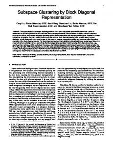
4.2 Theoretic efficiency In stage 1, the data is read in, normalised and placed into bins in such a way that the bin totals and the ids of the points in each bin can be retrieved. This is linear in N and D, O(N D). In stage 2, the bin totals are scanned and the dense areas flagged. This is better than linear by a constant factor. At this stage, the ND (noise only dimensions) are discarded. Stage 3 computes the degree of CD clustering between all the members of CD. This  2  involves operations. While this is potentially worst-case O(D2) the computation is a single pass over the points in the dense bins, typically a small fraction of N for any given dimension, and is thus very fast compared to typical clustering algorithms, which are rarely close to O(N) per clustering and may require repeated iterations. Thus this stage is sub-linear in N and sub-quadratic in CD. Stage 4, finds the maximal cliques. If the number of cliques is small or the cliques are relatively small and mainly disjoint, this operation is close to linear in CD. In most cases it will not significantly affect the overall efficiency by exceeding O(CD2). Having found the cliques, Stage 5, determining the clusters, is linear or log-linear in the number of points in the dense areas and CD. The complexity depends on the sorting technique used. If the number of classes per edge is small, then a linear hash technique is advised. Overall, therefore, assuming the maximal clique enumeration does not hit a ‘hard’ graph, the efficiency of the whole algorithm is O(N (D + CD2)). If the subspaces are relatively small, then the approach is strongly linear as reflected in our scaleup graphs (Figures 2 and 3). While two algorithms may have similar theoretic efficiency, 10 passes over the data or a complex operation on each pass takes much longer than a single low complexity pass and for a very large N, that can be exceedingly significant to the user. The great simplicity of this approach, where no stage takes more than a single pass and the operations are very simple, makes it highly suited to very large databases.

5.1 Accuracy Accuracy has two principal components: the accuracy of subspace determination and that of cluster recovery. For the first, we use precision and recall as they are usually defined. TP TP (1) Pr ecision( P) = ; Re call( R) = TP + FP TP + FN using true positives (TP) for the correctly identified dimensions, false positives (FP) for the dimensions erroneously identified and false negatives (FN) for the missed dimensions. For cluster or point accuracy we use the true positive and false positive rates for the cluster points and the Adjusted Rand Index (ARI) [48]. The ARI takes into account false and true positives and negatives and is thus a sound measure of clustering results on data for which we know the expected result. A perfect score is 1.0 (100%) and no correctness of partitioning receives 0.0 (0%). The ARI is based on the Rand Index [41] and measures how similar the computed partition V is to the actual clustering U. Denote a, b, c and d as the number of point pairs which are in the same cluster in U and V, in the same cluster in U but not in V, in the same cluster in V but not in U and in different clusters in both U and V. Then the ARI is defined as 2(ad − bc) (2) ARI (U ,V ) = (a + b)(b + d ) + (a + c)(c + d )

4.2 Memory usage Memory use is O(N D) but at no stage is there any need to hold information from more than two attributes in memory. If the database has an N that can be retained in memory by only pulling in two attributes at a time, then this is very efficient.

Precision, recall and ARI are presented throughout as percentages.

6

For disjoint clusters that are produced by some mechanism that approximates a normal distribution, the algorithm can produce almost any desired level of point true positives (TPR) for non-overlapping clusters by adjusting the expansion factor α (see section 3). Table 1 shows the effect of α on point TP and FP. Increasing α greatly increased TPR at a small cost in speed and the point FP rate. We found that TPR is always higher if we scale up α for larger cliques and higher N. We present accuracy results throughout the following Results sections.

Table 1. MAXCLUS res results ults for 50 dimensions with 2 disjoint 55-dimensional clusters and 20% noise. False positive rates are the highest collected from either the noise or the other cluster. *See text.

0.07

Subspace Precision & Recall 100%

Points: True Positives 98%

Points: False Positives 1 point

10,000

0.75

100%

98%

0.4%

100,000

10.7

100%

97%

0.18%

5.2 Scaling

100,000*

9.43

100%

71%

0.04%

5.2.1. Scaling by data size. The scaling results by the data size N verify that the algorithm is approximately linear in N (Table 1). 10,000 points with 50 dimensions, 10 of them containing clusters took under a second. Times included reading in the dataset from disk but not outputting a list of the clustered points to the disk though they do include computing accuracy rates from class numbers provided in the test dataset. This was also true

Table 2.1,000 Subspace accuracy and We experiments. pointsdetection took order 102 seconds. clustering point accuracy for 10,000 points with 2et present our results with these algorithms below. Parsons disjoint clusters each of 4,000 points and 10% of D al. in their review showed MAFIA and FindIt scaling dimensions, and 20% noise. approximately linearly with N with MAFIA completing its Points:resultsPoints: task at a speed close SubSpace to our MAXCLUS (though Time D computer CD Precision True False their specifications are not given) while FindIt (secs) & Recall Positives was about 10 times slower thoughPositives the gap narrowed on 98% is fast1 point very However, due to 50 large 10 datasets. 0.75 100% MAFIA aggressive pruning and FindIt due to97% sampling and [38] 100 20 1.8 100% 0% found a resulting loss of accuracy for both. In their 95% 200 40 4.94 100% experiments, both MAFIA and FindIt were not 0% able to identify the subspaces with full accuracy on a simple 87% 400 80 15.54 100% 0% synthetic dataset very similar to those used in our experiments. Obviously the many algorithms that require model fitting or various kinds of iterative methods will be too costly for large N though useful for certain domains.

N

Time (secs)

1,000

5.2.2. Scaling by Dimensionality. Theoretically, we expect the algorithm to scale linearly in D and by the quadratic of CD. Figure 2 shows a slight upward curve well below the worst-case theoretical, as we anticipated in our discussion of the theoretical complexity. Enumerating two cliques is obviously a very simple case so the Figure 3. Scaling by increasing dimensionality D. for all the algorithms in our comparison experiments. Our results show that finding the subspaces is strongly linear in N, the slight non-linearity comes from the final stage of extracting the points from the clustered dimensions. The last line in Table 1 illustrates the effect of collecting less aggressively (not increasing α). In all cases, the point false positive rate is close to zero despite a 20% noise level. For 100,000 points with 20,000 noise points, only about 30 noise points appeared in each 40,000 point cluster. This illustrates the expected strong suppression of randomness due to subspace size. Some papers report scaling results. The recent state-ofthe-art algorithm SSPC [46] showed approximate linear scaling with N but took order 105 seconds for a simple data set with 100K points as did PROCLUS in their

Figure 2. Scaling by increasing dataset size N.

7

PROCLUS an average of 10.48% with a best ARI of 74.34%. K Prototype had a best ARI of 49.14%. SSPC typically selected around 25 attributes for each of the clusters. A small subspace is generally more useful as a predictor than a large one. Another UCI repository dataset with all real valued attributes is chemical analyses of various types of glass [37]. There are 3 classes and 9 attributes. MAXCLUS achieved an ARI of 89.62% while we were unable to get a result with SSPC. Harp gave an ARI of 15.52% and PROCLUS an average of 22.51% with a best ARI of 54.54%. K Prototype had a best ARI of 27.16%. Even though the MAXCLUS ARI is good, the ability to separate the classes fell short of machine learning algorithms using some labeled training data. Examination of the dataset shows that only one attribute has more than one visible dense area in its distribution and this only allows one type of glass out of three to be distinguished which is essentially what MAXCLUS achieved. This is a very clear example of the limitations of unsupervised approaches in the case where the class distinctions cannot be detected without the help of additional dimensions (e.g. some labels). We wanted to test the algorithm on large datasets with higher dimensionality but there are very few such labeled datasets available and those that have many dimensions usually contain binomial attributes while MAXCLUS is currently intended for real or multinomial valued attributes. High dimensionality is easily found in genetic datasets but the number of instances is typically small. Adapting the algorithm to binomial data and small instance sets is ongoing. However, as discussed above, any dimensionality above 10 provides a serious efficiency challenge for current methods in addition to dealing with noise, both of which MAXCLUS successfully addresses.

hardness of that part of the problem has no effect here.

5.3 Noise Some authors report noise contamination results. Candillier et al [14] say that their method (SSC) has 90% purity in the presence of 20% noise and that LAC [17] has only 76%. They do not give results for different D or CD but as our results and simple probability theory can show, noise contamination should drop sharply with subspace size and, even at only 10 dimensions, for MAXCLUS this is effectively 0%. As each cluster is a noise contributor in its non-relevant dimensions for every other cluster covering those dimensions, noise levels of 90+% are often present without interfering with clustering accuracy. As SSPC is by far the best of the comparison algorithms and can handle noise we compared SSPC and MAXCLUS on two synthetic datasets. The first (D1) had 1200 points 3 clusters and no noise. The second (D2) had 2400 points, the same three 3 clusters and 50% noise. As SSPC does better on disjoint subspaces we used this type of cluster. MAXCLUS was run once on each dataset and achieved 99.8% ARI on D1 and 99.3% on D2. Subspace precision and recall were 100% on both runs. SSPC was run 10 times and the best result (achieved once out of 10) was 94.3% ARI on D1 and 59.3% on D2. Subspace precision and recall were 100% and 91.7% on D1 and 100% and 86.7% on D2 for these runs. These results show that MAXCLUS was little affected by noise while SSPC had a clear decline in its cluster identification accuracy.

5.4 Real datasets We used the Adjusted Rand Index [48] to assess the method’s performance on the Wisconsin Diagnostic Breast Cancer dataset [37]. It contains 569 complete records with 30 attributes and 2 classes, benign and malignant. The algorithm found several small subspaces with high ARI values up to 98%. Previously, a separation using SVMs achieved an estimated accuracy of 97.5% using repeated 10-fold cross-validations [32, 30]. This data is interesting because, like many real data sets, there is no visually obvious separation into two classes if one inspects the separate dimensions. However, the classes are linearly separable so an algorithm that follows a k-means approach and starts with two well-separated centroids, may, almost accidentally, do quite well. However, they fail to find any subspace information [17]. Since the benign cases are well clustered MAXCLUS readily identifies small subspaces in which a strong separation can be made. The best of the comparison algorithms, SSPC, achieved a mean ARI of 39.46% with a best result of 70.61% over 10 runs, HARP achieved an ARI of 58.54,

5.5 Comparing algorithms Table 3 lists the algorithms and their mandatory parameters (e.g. the final number of clusters, number of rounds of iteration), and whether they handle outliers and overlapping subspaces. Each algorithm may have many more non-mandatory parameters. CAST is the only algorithm not requiring foreknowledge of the final number of clusters but it has other more obscure parameters. None of the algorithms offer the novice user an easy means of clustering a dataset whose characteristics are largely unknown even if it has distinct clustering. Another major disadvantage of almost all the algorithms is that they are non-deterministic. Each run gives a different result. We report the best subspace accuracy we got but the average was much lower. The ARI reported is the mean and kPrototype, HARP and to a less extent SSPC showed quite wide variations on this though they never outperformed MAXCLUS. MAXCLUS is deterministic 8

Table 4. Subspace identification accuracy, cluster accuracy (ARI) and speed for various algorithms. Total dimensions D = 100, 4 disjoint clusters involving 24 dimensions, N = 1000 or 10,000 points and 20% noise.

making it reliable and very fast as only one iteration is needed. It also has no mandatory parameters, handles noise very well and detects overlapping subspaces and clusters. This makes it unique among all the algorithms we studied. Table 4 reports the accuracy and speed results we obtained for varying N. Clearly SSPC is the best of the comparison algorithms though it falls short of the accuracy of MACLUS and runs very much slower even when the relative speed of Java and C++ is taken into account. In fact, with execution time running into days, it proved impractical to test any of these algorithms on 100K points which MAXCLUS finished in a few seconds. Table 5 shows how the various algorithms respond to a doubling of the dimensionality, again MAXCLUS had the edge followed by DIANA and SSPC.

Algorithm DIANA CLARANS Kprototype CAST PROCLUS HARP SSPC BAHC MAXCLUS

Algorithm

Table 3. Subspace clustering algorithms and their mandatory parameters. N/a means there are optional parameter(s). DIANA CLARANS Kprototype CAST PROCLUS HARP SSPC

Other parameters N/a Yes N/a Yes Yes Yes Yes

Outliers handled No No No Yes Yes Yes Yes

Overlap allowed No No No No No No Yes

BAHC* MAXCLUS

Yes No

N/a No

N/a N/a

Yes Yes

No Yes

N/a N/a N/a N/a 57.6%* 35% 93.8%* N/a 100%

N/a N/a N/a N/a 55%* 86.7% 87%* N/a 100%

Speed 1K (secs) 59 100 99 417 552 135 277 40 0.63

Speed 10K (secs) 6045 956 2044 41136 3918 9941 2470 3816 3.54

ARI 21.2% 2.4% 23.3% 3.6% 35.2% 22.4% 80.9% 7.9% 99.5%

Table 5. Scaling with increased dimensionality for various algorithms. Total Total dimensions D = 100 (A) and 200 (B), 4 disjoint clusters involving 24 (A) and 48 (B) dimensions, N = 1000 points and 20% noise.

5.7 Overlapping subspaces and clusters

Nb. of rounds N/a N/a Yes Yes Yes N/a N/a

Subspace Recall

the ARI for the disjoint case was 99.6% while that for the overlapping case was 91.8% due to the expected small spurious cluster. However, 81% of these points had already been assigned to the 5-clique. If we introduce a weak exclusivity requirement, that is that each point is only allowed one cluster label for overlapping clusters (the largest subspace assigned first), then this spurious cluster disappears (drops below the minimum cluster size threshold) and our full accuracy is restored.

Where not obvious, mandatory parameters were set for the various algorithms based on the advice given by the authors in their papers and adjusted if the algorithm failed. MAXCLUS has no mandatory parameters. The adjustable internal constants are set as described in Section 3. Two parameters scale to the dataset as necessary and thus none need to be supplied by the novice user. The third, the noise threshold parameter, a fixed constant in our experiments, can also be adjusted by providing a few training examples of noise dimensions.

Nb. Of clusters Yes Yes Yes No Yes Yes Yes

N/a 10 10 10 10 N/a 10 N/a N/a

Subspace Precision

*Best result out of 10.

5.6 Parameter setting

Algorithm

Iterations

DIANA CLARANS Kprototype CAST PROCLUS HARP SSPC BAHC MAXCLUS

Iterations N/a 10 10 10 10 N/a 10 N/a N/a

Speed for A (secs) 59 100 99 417 552 135 277 40 0.63

Speed for B (secs) 86.14 190 250 929 891 553 430 105 0.81

Scaleup 1.46 1.90 2.53 2.23 1.61 4.10 1.55 2.63 1.29

If the overlap is smaller or both subspaces larger, this would of itself suppress the likelihood of a false cluster appearing. Over the course of many experiments we found that MAXCLUS handles subspace overlaps effectively. Virtually all algorithms to date have employed strong exclusivity – one cluster label assigned per input point. However, there are certainly cases where this is too strong. In a single microarray sample, there may be genes expressed from several different pathways – gene clusters. Thus providing choice over the exclusivity level – None/Weak/Strong is another powerful feature of MAXCLUS. SSPC is the only one of the comparison algorithms that can handle cluster overlaps. On this small but significant problem, SSPC correctly identified the subspaces on 2 out

Consider Figure 1 which has 3 subspaces, 2 overlapping. We tested this scenario in comparison with the same subspaces but where each one is disjoint. The 3clique which shares 2 dimensions with another clique is very likely to produce some dilution of accuracy as a spurious cluster containing points from the 5-clique can be found by chance in the 3-clique. This is what we observed. In fact, a small heavily overlapping subspace like this is the most difficult case. In both cases we achieved 100% precision and recall for the subspaces but

9

International Conference on Management of Data, pp. 94105, 1998.

of 10 attempts with a range of ARI values from 41.9% to 89.8%, which it achieved when finding the correct subspaces. SSPC is not deterministic due to its random seeds.

[3] C. C. Aggarwal, J. L. Wolf, P. S. Yu, C. Procopiuc, and J. S. Park. Fast algorithms for projected clustering. In Proc. of the ACM SIGMOD International Conference on Management of Data, pp. 61-72, 1999.

6. Conclusion and future work

[4] C. C. Aggarwal and P. S. Yu. Finding generalized projected clusters in high dimensional spaces. In Proc. of the 2000 ACM SIGMOD International Conference on Management of Data, pp. 70-81, 2000.

Our contribution here is a framework for subspace enumeration and clustering with several phases and in each phase one can use one of the panoply of existing approaches. We also present a very efficient example. Our experiments confirm that if a cluster is distinguishable from the noise background on its relevant dimensions, then those dimensions and the member points that lie in a collectible proximity to the cluster’s dense areas can be identified in an efficient and accurate way even if the space contains many noise points. The MAXCLUS algorithm, with no costly iterations and approximately linear scaling in N and D and usually sub-quadratic in CD, approaches the limit we can reasonably expect to achieve by any means without supervised training. The clustering part can be entirely parallelised as the clustering of each dimension pair is independent and, on huge databases, a random sample can be fed to the algorithm to further enhance the speed of finding the subspaces. If the clusters are well defined and separable on at least one attribute, then the algorithm can discover and separate them. We achieved a very high success rate in identifying subspaces and the cluster point true positive rate can also be very high with almost no false positives due to the advantages of dimensionality. If these criteria are not met, providing a number of training examples can allow the algorithm to improve its accuracy. In future work we will be looking at supervised and semisupervised clustering, use of binomial attributes and D >> N as in microarrays. Preliminary tests show that the algorithm can handle such data.

[5] Bansal, Nikhil, Blum, Avrim and Chawla, Shuchi. Correlation Clustering. Machine Learning, 56, 153–167, 2004. [6] Bellman, Richard, Adaptive Control Processes: A Guided Tour. Princeton University Press, 1961. [7] K Beyer, J Goldstein, R Ramakrishnan, and U Shaft. When is “nearest neighbour” meaningful? In Proc. of the Intl. Conf. on Database Theory (ICDT 99), pp. 217–235, 1999. [8] C. Bron and J. Kerbosch, Algorithm 457: Finding all cliques of an undirected graph, Commun. ACM, Vol. 16: 575--577, 1973. [9] E. Bingham and H. Mannila. Random projection in dimensionality reduction: applications to image and text data. In Knowledge Discovery and Data Mining, pp. 245250, 2001. [10] Amir Ben-Dor, Ron Shamir and Zohar Yakhini. Clustering Gene Expression Patterns. Journal of Computational Biology. Vol. 6 (3/4), pp. 281-297, 1999. [11] Y. Cheng and G. Church. Biclustering of expression data. In Proc. (ISMB’00), pp. 93-103, 2000. [12] C.-H. Cheng, A.W. Fu and Y. Zhang. Entropy-based subspace clustering for mining numerical data. In Proc. Of the 5th ACM SIGKDD International Conference on Knowledge Discovery and Data Mining, pp. 84-93, 1999. [13] J.-W. Chang and D.-S. Jin. A new cell-based clustering method for large, high-dimensional data in data mining applications. In Proc. of the 2002 ACM Symposium on Applied Computing, pp. 503-507, 2002.

7. Acknowledgement

[14] Laurent Candillier, Isabelle Tellier, Fabien Torre and Olivier Bousquet. SSC: Statistical Subspace Clustering. In Proc. Of Machine Learning and Data Mining in Pattern Recognition: 4th International Conference (MLDM’05), pp. 100-109, 2005.

The authors are supported by the National Science and Engineering Research Council of Canada (NSERC). We would like to thank Kevin Yip of Yale for providing executables for SSPC and the Biosphere project containing various algorithms.

[15] M. Dash, K. Choi, P. Scheuermann and H. Liu. Feature selection for clustering – a filter solution. In. Proceedings of the IEEE International Conference on Data Mining, pp. 115-122, 2002.

8. References

[16] C. Ding, X. He, H. Zha and H.D. Simon. Adaptive dimension reduction for clustering high dimensional data. In Proc. of the 2nd IEEE International Conference on Data Mining, pp. 147-154, 2002.

[1] D. Achlioptas. Database-friendly random projections. In Proc. of the 20th ACM SIGMOD-SIGACT-SIGART Symposium on Principles of Database Systems, pp. 274281, 2001.

[17] Carlotta Domeniconi, Dimitris Papadopoulos, Dimitrios Gunopulos, and Sheng Ma. Subspace clustering of highdimensional data, In Proc. of the 4th SIAM International Conference on Data Mining (SIAM’04), 2004.

[2] R. Agrawal, J. Gehrke, D. Gunopulos, and P. Raghavan. Automatic subspace clustering of high dimensional data for data mining applications. In Proc. of the ACM SIGMOD

10

[18] P. Drineas, A. Frieze, R. Kannan, S. Vempala and V. Vinay, Clustering Large Graphs via the Singular Value Decomposition. Machine Learning, 56, 153–167, 2004.

and Development in Information Retrieval( SIGIR 04), pages 218-225, 2004. [33] B. Liu, Y. Xia, and P. S. Yu. Clustering through decision tree construction. In Proc. of the 9th International Conference on Information and Knowledge Management, pp. 20-29, 2000.

[19] O. Dubois and G. Dequen. A backbone-search heuristic for efficient solving of hard 3-sat formulae. In IJCAI, pp. 248253, 2001. [20] X. Z. Fern and C. E. Brodley. Random Projection for High Dimensional Data Clustering: A Cluster Ensemble Approach. In Proc. of the 20th International Conference on Machine Learning (ICML 2003),Washington DC, USA, August 2003.

[34] A.A. Melkman and E. Shaham. Sleeved coClustering. In Proc. of the 10th ACM SIGKDD International Conference on Knowledge Discovery and Data Mining (KDD'04), pp. 635-640, 2004. [35] O.L. Mangasarian, W.N. Street and W.H. Wolberg. Breast cancer diagnosis and prognosis via linear programming. Operations Research, 43(4), pp. 570-577, 1995.

[21] J. H. Friedman and J. J. Meulman. Clustering objects on subsets of attributes. Journal of the Royal Statistical Society B, Vol. 66 (4), pp. 815-849, 2004.

[36] R. Ng and J. Han. Efficient and Effective Clustering Methods for Spatial Data Mining. In Proc. of the 20th VLDB Conference, pp. 144-155, 1994.

[22] Andrew Foss, Osmar R. Zaïane, A Parameterless Method for Efficiently Discovering Clusters of Arbitrary Shape in Large Datasets , in Proc. of the IEEE International Conference on Data Mining (ICDM'2002), pp 179-186, 2002.

[37] Newman, D.J. & Hettich, S. & Blake, C.L. & Merz, C.J. (1998). UCI Repository of machine learning databases, www.ics.uci.edu/~mlearn/MLRepository.html.

[23] M. R. Garey, R. L. Graham, D. S. Johnson and D. E. Knuth. Complexity Results for Bandwidth Minimization. In SIAM J. Appl. Math., 34:3, pp. 477-495, 1978.

[38] L. Parsons, E. Hague and H. Liu, Subspace clustering for high dimensional data: a review. SIGKDD Explorations, Vol. 6 (1), pp. 90-105, 2004.

[24] Ian P. Gent and Toby Walsh. The SAT phase transition. In Proceedings of the Eleventh European Conference on Artificial Intelligence (ECAI'94), pp. 105-109, 1994.

[39] C. M. Procopiuc, M. Jones, P. K. Agarwal, and T. M. Murali. A monte carlo algorithm for fast projective clustering. In Proc. of the 2002 ACM SIGMOD International Conference on Management of Data, pp. 418-427, 2002.

[25] S. Goil, H. Nagesh, and A. Choudhary. Mafia: Efficient and scalable subspace clustering for very large data sets. Technical Report CPDC-TR-9906-010, Northwestern University, 2145 Sheridan Road, Evanston IL 60208, June 1999.

[40] J. M. Pena, J. A. Lozano, P. Larranaga, and I. Inza. Dimensionality reduction in unsupervised learning of conditional Gaussian networks. IEEE Transactions on Pattern Analysis and Machine Intelligence, Vol. 23(6), pp. 590-603, June 2001.

[26] Z. Huang. Extensions to the k-means Algorithm for Clustering Large Data Sets with Categorical Values. Data Mining and Knowledge Discovery, Vol. 2 (3), pp. 283-304, 1998.

[41] W.M. Rand. Objective criteria for the evaluation of clustering methods. Journal of the American Statistical Association, Vol. 66, pp. 846-850, 1971.

[27] M.E. Houle and J Sakuma. Fast approximate similarity search in extremely high-dimensional data sets. In Proc. 21st International Conference on Data Engineering (ICDE 2005), pp. 619-630, 2005.

[42] V.S. Tseng and C-P Kao. Efficiently Mining Gene Expression Data via a Novel Parameterless Clustering Method. IEEE/ACM Transactions on Computational Biology and Bioinformatics, Vol. 2(4), pp. 355-365, 2005.

[28] Alexander Hinneburg , Daniel A. Keim, Optimal GridClustering: Towards Breaking the Curse of Dimensionality in High-Dimensional Clustering. In Proceedings of the 25th International Conference on Very Large Data Bases, pp.506-517, September 07-10, 1999.

[43] K.-G. Woo and J.-H. Lee. FINDIT: a Fast and Intelligent Subspace Clustering Algorithm using Dimension Voting. PhD thesis, Korea Advanced Institute of Science and Technology, Taejon, Korea, 2002.

[29] Y. Kim, W. Street and F. Menczer. Feature selection for unsupervised learning via evolutionary search. In Proc. of the 6th ACM SIGKDD International Conference on Knowledge Discovery and Data Mining, pp.365-369, 2000.

[44] Kevin Y. Yip, David W. Cheung and Michael K. Ng. A highly-usable projected clustering algorithm for gene expression profiles. In Proc. of the 3rd ACM SIGKDD Workshop on Data Mining in Bioinformatics (BIOKDD’03), pp. 41-48, 2003.

[30] L. Kaufman and P. J. Rousseeuw. An Introduction to Cluster Analysis. Wiley, 1990. [31] H. Liu and H. Motoda. Feature Selection for Knowledge Discovery & Data Mining. Boston: Kluwer Academic Publishers, 1998.

[45] Kevin Y. Yip, David W. Cheung and Michael K. Ng. HARP: A Practical Projected Clustering Algorithm, IEEE Transactions on Knowledge and Data Engineering (TKDE), Vol. 16 (11), pp. 1387-1397, 2004.

[32] Tao Li, Sheng Ma, and Mitsunori Ogihara. Document Clustering via Adaptive Subspace Iteration. In Proc. of the 27th International ACM SIGIR Conference on Research

[46] Kevin Y. Yip, David W. Cheung and Michael K. Ng, On Discovery of Extremely Low-Dimensional Clusters using Semi-Supervised Projected Clustering, In Proc. of the

11

[50] J. Yang, W. Wang, H. Wang, and P. Yu. δ-clusters: capturing subspace correlation in a large data set. In Proc. 18th International Conference on Data Engineering, pp. 517-528, 2002.

IEEE International Conference on Data Engineering (ICDE’05), pp.329-340, 2005 [47] L. Yu and H. Liu. Feature selection for high-dimensional data: a fast correlation-based filter solution. In Proc. of the 20th International Conference on Machine Learning, pp. 856-863, 2003.

[51] Jiong Yang, Haixun Wang, Wei Wang, Philip S. Yu: Enhanced Biclustering on Expression Data. In Proc. of the 3rd IEEE Conference on Bioinformatics and Bioengineering (BIBE), pp. 321-327, 2003.

[48] K. Yeung and W. Ruzzo. An empirical study on Principal Component Analysis for clustering gene expression data. Bioinformatics, Vol. 17 (9) pp. 763-774, 2001.

[52] Zhang, Y., Abu-Khzam, F. N., Baldwin, N. E., Chesler, E. J., Langston, M. A., and Samatova, N. F. 2005. GenomeScale Computational Approaches to Memory-Intensive Applications in Systems Biology. In Proceedings of the 2005 ACM/IEEE Conference on Supercomputing, pp. 12, 2005.

[49] Kevin Y. Yip, Peishen Qi, Martin Schultz, David W. Cheung, and Kei-Hoi Cheung. SemBiosphere: A Semantic Web Approach to Recommending Microarray Clustering Services. In Proc. of the Pacific Symposium on Biocomputing, pp.188-199, 2006. http://yeasthub2.gersteinlab.org/sembiosphere/index.jsp.

12