A Spherical Robot-Centered Representation for Urban Navigation Maxime Meilland, Andrew I. Comport and Patrick Rives
Abstract— This paper describes a generic method for visionbased navigation in real urban environments. The proposed approach relies on a representation of the scene based on spherical images augmented with depth information and a spherical saliency map, both constructed in a learning phase. Saliency maps are built by analyzing useful information of points which best condition spherical projections constraints in the image. During navigation, an image-based registration technique combined with robust outlier rejection is used to precisely locate the vehicle. The main objective of this work is to improve computational time by better representing and selecting information from the reference sphere and current image without degrading matching. It will be shown that by using this pre-learned global spherical memory no error is accumulated along the trajectory and the vehicle can be precisely located without drift.
I. I NTRODUCTION Autonomous navigation in complex urban environments, including traffic and large scale distances is an active field in robotics and in particular precise localization of the vehicle is a very important aspect. Indeed, robust localization, particularly in urban canyons, is a non-trivial problem due to GPS masking and poor precision of low cost units. Classical dead reckoning methods like odometry, typically performed by inertial sensors and wheels encoders are prone to drift and therefore are not suited to large distances. Relatively recent performance improvements in computing hardware have, however made real-time computer vision suitable for intelligent vehicles. Visual odometry, which estimates the full 6 degrees of freedom (dof) of vehicle motion from image sequences produces very precise results and has lower drift than the most expensive IMU’s [12]. Feature-based methods (e.g. [12], [8], [19]) rely on an intermediary estimation process based on threshold detection ([10], [17]) before requiring matching between frames to recover camera motion. This feature extraction and matching process is often badly conditioned, noisy and not robust, and therefore it must rely on higher level robust estimation techniques and on filtering. Appearance and optical flow-based techniques are imagebased and minimize errors directly between image measurements. Methods such as [4] and [2] use a planar homography model, so that perspective effects or non-planar objects are not considered. Recent work [6], [7] uses a stereo rig and a quadrifocal warping function which closes a non-linear This work was supported by CityVIP ANR project M. Meilland and P. Rives are with INRIA Sophia-Antipolis, France
{Maxime.Meilland,Patrick.Rives}@inria.fr A. Comport is with CNRS, I3S laboratory Sophia-Antiplis, France
[email protected]
iterative estimation loop directly with images. This method leads to robust and precise localization. Visual odometry methods are however incremental and prone to small drifts, which when integrated over time become increasingly significant over large distances. In a similar way, simultaneous localization and mapping approaches [8], [16] allow both localization and cartography, giving alternative and promising solutions. Classically based on the Extended Kalman filter, these techniques have limited computational efficiency (inversion of a large covariance matrix) and cannot be used in real-time for very long trajectories. Moreover, they are subject to problems of consistency due to the linearization of the models. A solution to minimize drift is to use image-based memory techniques [18], [15], [20] where each position estimate is computed with respect to a reference image that has been acquired during a learning phase. An image-based memory is directly extracted from the image sensor and can be used to minimize an online image to recover camera position. In [5], a panoramic image memory is used combined with depth information extracted from a laser scan. Normally, direct image-based techniques use all the information contained within a target region but in fact, only a small part of this information is significantly important for the estimation process [3]. One of the objectives is therefore to prove that it is possible to obtain estimation results that have the same properties (precision, convergence, robustness...) with a lower computation cost by using just a subset of the information provided by images. Classically, edge and feature extraction techniques such as [10], [17], [21] are efficient in selecting useful information but work in a 2D image space and do not deal with 3D scene structure. On the other hand, saliency maps [14] often need prior knowledge of the environment. In [11], quadrangular textured primitives are extracted from the environment for robust indoor navigation. The structure of the scene is involved, but only vertical planes are extracted. Our goal is to extract information well adapted for navigation without supposing any prior knowledge of the 3D environment dynamics. Section IV describes a new pixel selection method that is based on both, image grey level variation and geometric structure influence on optimal localization and navigation, by choosing 3D pixels which best condition the 6 degrees of freedom of the vehicle. II. S PHERICAL R EPRESENTATION Assuming that during a learning step a lot of data has been acquired, the main problem is then to pre-process and store these data for further use. Building 3D CAD models as
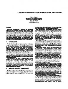
Fig. 1. Spherical representation: grey levels and their corresponding depths projected on a unit sphere S 2 .
intermediate representations introduce reconstruction errors and photometric inconsistences. Differences between the real images acquired online and the virtual ones resulting from the projection of an approximate 3D model induces errors and yields to a bad localization quality. To minimize global reconstruction and matching errors, it is necessary to have a model that reproduces, as close as possible, the real sensor measurements. Direct image-based models should therefore provide good photometric realism as an output result. An image-based memory is a good way to respect that constraint because it does not deviate far from the original sensor measurements used to build the model. Previously image memory approaches have used perspective images with a small field of view which are not well suited to recovering large motion differences between learning and online trajectories because of poor overlap. A wide view sensor is well adapted to do that, but classical omnidirectional cameras have poor resolution in most directions, and localization precision directly relies on that. We propose a spherical representation constructed from multi-perspective panoramic cameras so as to provide high resolution in all directions that is also augmented with a dense depth map. In order to have a generic model, a unit sphere is chosen to represent images. To obtain precise and unbiased results, spheres are sampled using the hierarchical isolatitude equal area partitioning given in [9]. This partitioning avoids oversampling and image distortion on poles which arise when a sphere is sampled using constant angles. It is also efficient for computing multiresolution view spheres because lower resolutions can be directly computed from base resolutions, while retaining equal area properties. We can see in Section III-D that a multi-resolution technique greatly improves the computational efficiency and expands the domain of convergence of the tracking method. Here the optimization problem is formulated as a pose estimation problem, that is directly related to the grey level brightness measurements and the 3D geometric configuration of the scene. Consequently, the spherical memory needs to be augmented with depth information. This depth information is extracted from dense matching between stereo cameras and/or laser scans. The global spherical robot centered representation is composed of full view geolocated spheres defined by S = {I, P} where I are the pixel intensities and P the associated 3D points (see Fig. 1).
The full collection of spheres is stored in a GIS (Georeferenced Information System), which is then used during the navigation phase. Our spherical representation presents some advantages : • Genericity allows combination of different kinds of sensors like perspective cameras, multi-view cameras or omnidirectional cameras and laser range finders. • All local view directions are provided for localization. • Full-view sensors well condition the observability of 3D motion [1] which greatly improves robustness. • Only one sphere suffices to recover different navigation directions, such as the two directions of a street. • Photometric consistence between the spherical image and the online sensor, enhances the performance of image-based techniques. III. E FFICIENT AND ROBUST L OCALIZATION It is considered that during navigation, a current image b = (R, b b I and an initial guess T t) ∈ SE(3) of the current b ∈ SO(3) is a rotation vehicle position are available, where R 3 b matrix and t ∈ R is a translation vector. This initial guess permits extraction of the closest reference sphere S ∗ from a database of spheres. A superscript ∗ will be used in the remainder to designate reference view variables. The function w(P ∗ , T, K) is defined to represent the motion of 3D points of a reference sphere w.r.t. the current camera motion. This motion model is a spherical warping that is detailed in Section III-A, where T is the true current camera pose and K ∈ R3×3 is the upper triangular intrinsic parameter matrix of the current sensor, which does not vary with time and is assumed implicitly given. The current image is warped to the reference sphere by: ¢¢ ¡ ¡ (1) I ∗ (P ∗ ) = I w P ∗ ; T , ∀P ∗ ∈ S ∗ .
b of the current camera It is assumed that an initial guess T pose with respect to the reference sphere is available. The tracking problem is then to estimate the incremental pose b = T. Using an iterative optimization T(˜ x) such that T(˜ x)T scheme, the estimate is updated at each step by an homogeb ← T(x)T. b The unknown 6 degrees neous transformation T of freedom parameters, x ∈ R6 , are defined as: Z 1 (ω, υ)dt ∈ se(3), (2) x= 0
which is the integral of a constant velocity twist which produces a pose T. The pose and the twist are related via the exponential map as T = e[x]∧ , where the operator [.]∧ is defined as follows: · ¸ [ω]× υ [x]∧ = , (3) 0 0
where [.]× represents the skew symmetric matrix operator. Thus, the current camera pose can be estimated by minimizing a non-linear function: ´ ´2 X ³ ³ b − I ∗ (P ∗ ) . (4) I w(P ∗ , T(x)T) O1 (x) = P ∗ ∈S ∗
P*
q*
Where JI ∗ is the reference image gradient on the sphere with respect to spherical coordinates (θ, φ) of dimension n × 2n, Jw is the derivative of spherical projection of Equation (5) of dimension 2n × 3n, and JT depends on the parameterization of x with a dimension of 3n × 6 from Equation (2). The vector of unknown parameters x is obtained iteratively from: x = −λ(JT J)−1 JT (I − I ∗ ), (8)
K[R | t ]
O
p
S*
I
(R,t)
Fig. 2. Spherical warping of a perspective image. S ∗ is the reference sphere. I is the image plane.
where (JT J)−1 JT is the pseudo-inverse J+ of the matrix J and λ is the tuning gain which ensures an exponential decrease of the error.
A. Spherical Warping
C. Robust Estimation
A spherical warping is based on the projection of a point P ∈ R3 on the unit sphere:
While navigating in an urban context, the environment can vary between the reference and the current images due to moving vehicles, pedestrians, specular reflections or self occlusions of buildings perceived from different viewpoints. To deal with these changes, a robust M-estimator is used and included in the objective function (4) which becomes: Ã ! ³ ´ X ∗ ∗ ∗ b O2 (x) = ρ I w(P , T(x)T) − I (P ) .
q=
P ∈ S2 . kPk
(5)
It is proposed here to work in spherical coordinates (θ, φ, ρ), because a spherical image sensor is over-parameterized in Cartesian space, especially its images derivatives. If we define q = (x, y, z), its corresponding spherical coordinates are: ρ cos(θ) sin(φ) x , y = ρ sin(θ) (6) ρ sin(θ) cos(φ) z
where ρ in this case equals 1 (unit sphere). Consider T = (R, t) to represent the homogenous rigid transformation between the pose of the current image with respect to the reference unit sphere. To warp current image grey levels to the reference sphere, reference points P ∗ have to be projected onto the current image with a 3 × 4 perspective projection matrix M = K[R|t] ∈ R3×3 ×SE(3). The homogeneous vector p = (u, v, 1)T ∈ P(3) in pixel coordinates is given by p = MP. Then current image I grey levels are interpolated at points p to obtain corresponding intensities in spherical coordinates. The case presented here is for perspective cameras. For omnidirectional cameras only the projection matrix M = K[R|t] differs in the warping. B. Minimization The aim is to minimize the objective criteria (4) in an accurate, robust and efficient manner. Since this is a nonlinear function of the unknown pose parameters, an iterative minimization procedure can be used. The objective function is minimized by ∇O1 (x)|x=˜x = 0, where ∇ is the gradient operator with respect to the unknown x defined in equation (2) assuming a global minimum can be reached in x = x ˜. It is possible to use either the efficient second order approximation (ESM) from [4] or a first order approximation depending on the computational resources available. In case of using a first order approximation, the Jacobian can be decomposed into modular parts as: J(x)|x=˜x = JI ∗ Jw JT .
(7)
P ∗ ∈S ∗
(9) In this case (8) becomes x = −λ(DJ)+ D(I − I ∗ ) with D the diagonal weighting matrix computed via a robust weighting function [13]. D. Multi-Resolution Reference Sphere To improve the computational time and the convergence domain, a multiresolution approach is considered. Each sphere is under-sampled N times (depending on the original sphere size) by a factor of 2. This factor is imposed by the HEALpix partitioning scheme [9], because available equal area resolutions are in 2k . The minimization begins at the lower resolution, and the result is used to initialize the next level repeatedly until the higher resolution is reached. In this way, larger displacements are minimized at low cost on smaller images. Under-sampling produces smoothed images so strong edges, which provide more accuracy in alignment are only used in higher resolutions, when the current estimate is close to the solution. Local minimas can also be avoided in this way. Current images also need to be resampled, to keep the same angular resolution than the reference sphere. IV. I NFORMATION S ELECTION The essence of appearence-based methods is to minimize pixel intensities directly between images. Images are, however, clearly redundant, i.e. a lot of information is not overly important for navigation, such as completely untextured parts. This kind of information should not be used for several reasons. One of them is that if spheres are constructed from a panoramic multi-camera at high resolution, the number of pixels to warp at each iteration of the minimization process could be extremly large. Therefore reducing the dimension is essential for real-time computing.
Fig. 4.
Fig. 3. Spherical saliency maps associated with the six degrees of freedom of the vehicule. Important values are in white. J1 , J2 , J3 are the translational components. J4 , J5 , J6 are the rotational components.
A classic approach is to select only the best corners or edges (intensity gradients) in grey-level images, by using a feature detector [10], [17]. This na¨ıve approach does not consider the importance of the structure of the scene and can lead to the selection of non-observable measurements. For example, selecting high intensity gradient points at infinity, rather than more informative but low gradient close points in a scene, will yield imprecise results. In the worst case it will not even be possible to estimate translation because of the invariance of infinite points in pure translation. At the same time infinite points are also useful because they improve the stability and robustness of the tracking algorithm due to their small displacement in the images for large translations. The difficulty is therefore to analyse the accuracy and robustness of selected points. In [3], only linear or quadratic subsets are extracted for template-based tracking. Such subsets are good for linear convergence allowing to converge quickly. Unfortunately, this method suggests rejecting strong edges which are essential for obtaining good precision. The novelty of the approach proposed here is to quantify the effect of the geometric structure and the image intensity measurements on navigation by analyzing directly the entire analytical Jacobian which relates scene movement to sensor movement. The aim being to select points which best condition the six degrees of freedom of the vehicle. Indeed, the Jacobian directly combines grey level gradient (image derivatives) and geometric gradient. More precisely, the reference Jacobian matrix of the spherical projection in equation (7), can be decomposed into six parts corresponding to each degree of freedom of the vehicle with J = {J1 , J2 , J3 , J4 , J5 , J6 }. Each column Jj can be interpreted as a saliency map (see Fig. 3). A subset 1 2 3 4 5 6 of the entire set of pixels J = {J , J , J , J , J , J } ⊂ J is sought such that J is the reduced p × 6 version of J of dimension n × 6 with p ≪ n, where n is the number of points on the full sphere, and the rows of J are given by: ˜ Jk = arg max(Jji \ J),
(10)
j
which this corresponds to selecting an entire line i of J according to the maximum gradient of one column (direction)
Multi-resolution spherical saliency maps
TABLE I C OMPUTATIONAL TIME USING SALIENCY SELECTION % of bests pixels 100 75 50 25 Estimation time (ms) 203 34 21 16 Number of iterations 26 10 8 10
˜ ⊂ J is a j and where k is the next line that is added to J. J ˜ indicates intermediary subset of Jacobian that is sought. \J that it is not possible to reselect the same row. i.e. the lines ˜ until the of Jj are recursively chosen and inserted into J required number of lines have been selected, in which case it becomes J: i h 1 6 ⊤ J = J ,...,J . (11)
In the recursive selection process, the criteria (10) is applied iteratively in each direction such that an equal number of maximum gradients are chosen for each degree of freedom. In this way the pixels that have been chosen at the end of this algorithm are those that best condition each dof in the pose estimation process. Table I illustrates the computational time and number of iterations vs the number of salient pixels selected, for a 6 dof estimation run on simulated data. The algorithm stops when the error is less than 5%. It can be seen that both the number of iterations and computational time decrease with the number of pixels. Offline, all the pixels on the entire sphere are ranked according to criteria (10). This allows to precompute the pixel ranking and avoid costly computation during tracking. Online, the saliency map J is then constructed from the precomputed map by taking into account the camera viewpoint. Since the spherical representation is made of multiresolution spheres, the selection is computed at each scale. A new multi-resolution set of saliency maps is then obtained (see Fig. 4) and added to database. V. R ESULTS
A. Simulations A synthetic urban environment has been created (see Fig. 1). It contains textured corridors, infinite planes, etc... Corresponding depths are directly computed from the simulator. The trajectory of the camera is planned manually, a first learning step is realized at 1Hz at a speed of 2.5 m/s, providing a set of reference spheres with grey levels and depths in a global reference frame. Then a different trajectory of 150m is computed with a monocular camera at a frame rate of 25Hz. Although only simulated data is used here, there are still added noise and artifacts due to aliasing
Fig. 5. Blue circles indicate the position of reference spheres, black lines represent the environment structure. The estimated trajectory appears in red.
and texture mapping of the rendering engine (OpenGL). Nevertheless, this noise is correctly handled by the robust outlier rejection process and does not affect ground truth accuracy too much. In Fig. 5, the vehicle starts at position (X = 0, Z = −7) and follows the corridor. At that point a deviation is introduced in its trajectory to simulate obstacle avoidance or a vehicle overtaking. Following this, the vehicle goes around the round-about and returns in the opposite direction back to the starting point. Only the best N/10 points contained in the current warped sphere where used for the estimation. Even if the learning trajectory was different, the tracker was able to precisely locate the vehicle with an average error of 3cm. One advantage of a spherical representation can be seen, since the same spheres were used along the corridor in both directions. B. Experiments with a Real Sequence The algorithm was tested on a full-scale sequence1 which was acquired at the INRIA Sophia-Antipolis site. It contains buildings, vegetation, parked cars and pedestrians. A first learning loop of 260m was carried out using stereo images of 640×480 pixels in size and acquired with a frequency rate of 20Hz. This trajectory contains straight sections, corners and several hills (about 10m in height). It can be noted that the 6 degrees of freedom of the vehicle are required in this sequence. To obtain the reference trajectory and build the reference spheres, the quadrifocal odometry method from [7] was used in an offline phase with stereo images. The resulting reference trajectory is then obtained with a final error of 80cm at the loop closing point. The reference spheres are then sampled along the trajectory. The strategy is to select a sphere every 1.2 meters in straight sections. In turns, spheres are more densely sampled so as to recover overlap with stereo learning sequence. Such cases appear due to the small field of view of the camera sensor, around 85◦ , and significant displacement in the images during rotation. To build the spheres, the depths are directly obtained by triangulating from dense correspondences between the stereo images. The final set of reference spheres is shown in blue in Fig. 6. Although 1A
video of this experiments is attach to that paper and also available at http://www-sop.inria.fr/arobas/videos/spherical tracking.mp4
the reference positions of the spheres seem good, there are several matching errors which lead locally to a wrong positioning of the spheres. This is mainly due to the bad observabilty of some scene viewpoints, as well as errors and occlusions in dense correspondences. This leads to an error in the global positioning of the current vehicle during the learning run, and the estimated online trajectory contains discontinuities. A better learning step (i.e local positioning of the reference spheres, a full view sensor with higher resolution) may further improve the results and will allow to reduce the total number of spheres. A new trajectory is then obtained using a monocular camera to acquire images. To check the robustness of the method the path followed by the vehicle was slightly different from the reference one, global illumination changed, and some cars had left the parking lot. Two estimations of the trajectory were performed: the first one using all available information in the reference spheres and the second one using information selection from section IV with a ratio of N/4, where N is the total number of available points at each warping. Reducing the number of points by a factor of 4 directly divides the computational time by 4, which is not negligible. The resulting estimated trajectories are shown in Fig 6. The starting point is (0, 0) and the vehicle begins to move in positive Z direction. It can be seen that up until position (X = 20, Z = 80), the two trajectories are very similar, showing that proposed technique for selecting interesting pixels for navigating does not degrade the estimation. After that position, the red and green trajectories present slight differences. In that region the depths and the location of the spheres are unfortunately noisy, because the reference information is too far from the current view (images contain road, parked cars and vegetation), disparities were not accurate leading to an incorrect localization of the vehicle. Despite of some discontinuities due to errors on the reference spheres, the global trajectory represents the true trajectory accurately enough and proves that the presented method was able to track a different trajectory. The selection of information makes the algorithm faster without loosing accuracy and the estimated result seems to be smoother and contains less errors than the first one. Fig. 7 shows the input and output images used for the estimation of a particular position in the trajectory. The vertical black parts of the weight image (Fig. 7(c)) correspond to occlusions in the dense correspondences and are not used during minimization. Moving pedestrians and specular reflections on windows are correctly handled by the robust outlier rejection and appear in a dark color. Fig. 7(e) represents the information which was used for the second estimation (with saliency) and selected information (brighter) corresponds to visible salient parts of the world. VI. C ONCLUSIONS AND F UTURE W ORK The spherical robot-centered representation described here, is a generic model that could be used to localize a vehicle equipped with different kinds of image sensors. The
(a)
(b)
(c)
(d)
(e)
(f)
Fig. 7. Images used for the estimation of one incremental pose. Only interesting parts of spherical images are plotted. 7(a) Spherical reference image. 7(b) Current perspective image. 7(c) The robust weights. 7(d) The final error. 7(e) The saliency map extracted for the current position. 7(f) The robust weights with saliency selection
Fig. 6. Trajectory tracking in a 280m loop. The blue circles indicate the position of reference spheres; the estimated trajectory using all the image’s information appears in red ; the estimated trajectory using only best N/4 saliency information appears in green. It can be seen that when the two estimated trajectories are very close only one is visible
spherical representation has proved useful for storing all local information around a viewpoint. in particular, just one sphere covers a large domain, including different navigation directions. The selection of interesting pixels makes the localization faster and real-time computation possible. Future work will be devoted to determining an optimal set of spheres to store in the database which represent the environment in an optimal manner rather than sampling spheres with a constant step in the world. Another perspective will be to update the database with an online SLAM technique, in order to deal with changing environments. Using different kinds of sensors could potentially improve robustness and it will be interesting to study which sensor or set of sensors provides the best results. R EFERENCES [1] P. Baker, C. Fermuller, Y. Aloimonos, and R. Pless. A spherical eye from multiple cameras. In IEEE Conference on Computer Vision and Pattern Recognition, 1:576, December 2001. [2] S. Baker and I. Matthews. Equivalence and efficiency of image alignment algorithms. In IEEE Conference on Computer Vision and Pattern Recognition, volume 1, page 1090, December 2001. [3] S. Benhimane, A. Ladikos, V. Lepetit, and N. Navab. Linear and quadratic subsets for template-based tracking. In IEEE Conference on Computer Vision and Pattern Recognition, pages 1–6, June 2007. [4] S. Benhimane and E. Malis. Real-time image-based tracking of planes using efficient second-order minimization. In IEEE/RSJ Conference on Intelligent Robots and Systems, September 2004. [5] D. Cobzas, H. Zhang, and M. Jagersand. Image-based localization with depth-enhanced image map. In IEEE/RSJ Conference on Intelligent Robots and Systems, pages 1570–1575, September 2003.
[6] A.I. Comport, E. Malis, and P. Rives. Accurate quadrifocal tracking for robust 3d visual odometry. In IEEE Conference on Robotics and Automation, pages 40–45, April 2007. [7] A.I. Comport, E. Malis, and P. Rives. Real-time quadrifocal visual odometry. In The International Journal of Robotics Research, 29(23):245–266, February 2010. [8] A.J. Davison and D.W. Murray. Simultaneous localization and mapbuilding using active vision. IEEE Transactions on Pattern Analysis and Machine Intelligence, 24(7):865–880, July 2002. [9] K. M. Gorski, E. Hivon, A. J. Banday, B. D. Wandelt, F. K. Hansen, M. Reinecke, and M. Bartelman. Healpix – a framework for high resolution discretization, and fast analysis of data distributed on the sphere. The Astrophysical Journal, 622:759–773, 2005. [10] C. Harris and M. Stephens. A combined corner and edge detector. In Proceedings of the 4th Alvey Vision Conference, pages 147–151, 1988. [11] J.B Hayet. Contribution a` la navigation d’un robot mobile sur amers visuels textur´es dans un environnement structur´e. PhD thesis, LAAS, 2003. [12] A. Howard. Real-time stereo visual odometry for autonomous ground vehicles. In IEEE/RSJ International Conference on Intelligent Robots and Systems, September 2008. [13] P.J. Huber. Robust Statistics. New york, Wiley, 1981. [14] L. Itti, C. Koch, and E. Niebur. A model of saliency-based visual attention for rapid scene analysis. IEEE Transactions on Pattern Analysis and Machine Intelligence, 20:1254–1259, October 1998. [15] M. Jogan and A. Leonardis. Robust localization using panoramic view-based recognition. In IEEE Conference on Pattern Recognition, 4:4136, September 2000. [16] K. Konolige and M. Agrawal. Frameslam: from bundle adjustment to realtime visual mapping. IEEE Transactions on Robotics, 24(5):1066– 1077, October 2008. [17] D.G. Lowe. Distinctive image features from scale-invariant keypoints. International Journal of Computer Vision, 60(2):91–110, 2004. [18] M. Menegatti, T. Maeda, and H. Ishiguro. Image-based memory for robot navigation using properties of omnidirectional images. Robotics and Autonomous Systems, 47(4):251 – 267, 2004. [19] D. Nist´er, O. Naroditsky, and J. Bergen. Visual odometry. In IEEE Conference on Computer Vision and Pattern Recognition, volume 1, pages 652–659, July 2004. [20] A. Remazeilles, F. Chaumette, and P. Gros. Robot motion control from a visual memory. In IEEE International Conference on Robotics and Automation, volume 4, pages 4695–4700, April 2004. [21] J. Shi and C. Tomasi. Good features to track. In IEEE Conference on Computer Vision and Pattern Recognition, pages 593–600, June 1994.