preparing for validation of the model. This process also aids in establishing confidence on forecasting of future result
Sixth International Conference on Machine Learning and Applications
A Spline Based Regression Technique on Interval Valued Noisy Data Balaji Kommineni, Shubhankar Basu and Ranga Vemuri Department of ECE University Of Cincinnati {komminb,basusr,ranga}@ececs.uc.edu
Abstract
nique to model interval valued data. In their work, the authors use the correlation and covariance metrics to generate the regression models from the center values of the intervals. The model coefficients were then applied to the lower and upper bounds of regressors to predict bounds for the dependent variables. The drawback of the method by Billard and Diday is that it does not use the range information effectively. This causes failure in estimating the dependent variables where the bounds are not necessarily dependent on the respective bounds of the regressors. De Carvalho et al. [2] presented a solution to improve the results over Billard’s approach. Carvalho et al. use both the center and range information of the regressor intervals (CRM) to perform two independent regressions for the center and range of the dependent variable. The lower and upper bounds could then be computed by combining the predicted center and range values. This method showed a significant improvement over the method proposed by [3]. Both the methods above [3, 2] use the linear least square regression techniques.
In this paper we present a Spline based Center and Range Method (SCRM) to perform regression on interval valued noisy data. The method provides a fast and accurate mechanism to model and predict upper and lower limits of unknown functions in a bounded design space. This technique is superior to previously existing techniques like center and range linear least square regression (CRM). The accurate models may find wide usage in high precision applications. The effectiveness of the proposed technique is demonstrated through experiments on datasets with various applications.
1 Introduction Regression plays an essential role in engineering and scientific problems to model systemic behavior. This reduces expensive mathematical computation time. However in many current engineering problems simple linear regression techniques fail to capture the behavior accurately. This is attributed to non-linear system behavior and noisy and unstructured measured data. This requires an improvement in regression techniques that can capture the randomness resulting from noise. Introduction of noise in precision applications necessitate a measure of performance deviation from the nominal value. This can be achieved by an interval valued data set, where noisy data can be represented as intervals. An interval data classifies the lower and upper bound corresponding to worst and best performance possible. Thus, the problem at hand is changed from modeling real valued data to modeling intervals. But, there are some inherent problems with interval arithmetic. These make direct modeling on interval valued data unreasonable. The major shortcoming as explained by Moore [5] is expansion due to dependency. This causes undue increase in the width of the results, making them useless for real applications. Thus, a more sophisticated approach is needed for handling interval valued data. Billard and Diday [3] introduced a new regression tech-
0-7695-3069-9/07 $25.00 © 2007 IEEE DOI 10.1109/ICMLA.2007.100
Linear least square regression technique with lower order polynomials is an insufficient method to model nonlinear engineering system behavior. Very high-order polynomial regression, on the other hand, not only increases the dimensions of modeling but also suffer from multicollinearity. In this work we propose to improve the CRM method by using spline regression to fit the interval valued noisy data. Spline regression is a piecewise approximation based scheme which solves a set of equations to generate a perfect fit to the model data. This provides a much better accuracy compared to a very high order polynomial regression. It may be noted however that the spline regression is applicable to systems where the design space is bounded. For engineering and several other scientific applications this information is well defined, and therefore spline offers a better solution. The SCRM method uses Duchon pseudocubic spline [1] to regress over the center and range data. We use the root mean squared error and the square of correlation coefficient to prove the effectiveness of our method. The rest of the paper is organized as follows. Section 2 gives the motivation behind the work. Section 3 presents the SCRM technique and Duchon pseudo-cubic spline. In
241
Higher-order polynomial regression is an extension of linear regression. The polynomial equation is capable of capturing some regular non-linearity through a higher order term. However they are mathematically linear with respect to the modeling coefficients. For a univariate regression over an independent variable ’x’, a polynominal regression of order ’n’ can be mathematically represented as shown in Equation. (2).
30 Original
Least Squares
Polynomial
Spline
20
Y = X * SIN ( X )
10
0
−10
Y = β0 + β1 x + β2 x2 + ... + βn xn + "
−20
"Splineregression is a general technique for fitting and smoothing the twists and turns of a time line” [4]. Spline regression employs a piecewise solution of segments (expressed as dummy variables); it jumps to the next segment without an innapropriate break in two subsequent regression lines by joining knots . Higher order splines are used to fit data very smoothly yet flexibly. Splines find a much wider applicability for precision model fiting of nonlinear, sparse and unstructured data. Mathematically a linear spline regression model of order ’1’ can be expressed as in Equation. (3), where xi , xj are the independent variables, Yi is the dependent variable and bj represents the model coefficients and φ() represents a dummy variable.
−30
10
15
20
25
X
Figure 1. Modeling xsinx function using linear least square, polynomial and spline regression
Section 4 we discuss the experimental setup followed by the results in Section 5. Finally Section 6 provides the conclusion for this work.
(2)
2 Motivation Yi = In this section we compare the modeling technique using linear least square (polynomial) and spline regressions. We use the example of a non-linear mathematical function xsinx to demonstrate the effectiveness of using spline regression over linear regression techniques.
2.1
Linear Least Square vs. gression
bj φ(xi − xj ) + "
(3)
j
Detailed discussion of the particular class of spline regression making use of basis function is discussed in the next section. We now illustrate the accuracy of spline regression fit compared to linear least square regression using various polynominal orders. We apply these techqniues to the mathematical function y = x∗sin(x) which is a non-linear function in ’x’. For experimental purposes, we allow ’x’ to take any positive real values. Figure 1 shows the plot of polynomial linear least square regression (order one and four), and spline linear regression over data collected for the above mathematical function. The plot illuatrates that spline provide a perfect fit of the data with a negligible error as compared to significant errors for the other techniques.
Spline Re-
Linear least square regression is probably the most widely used regression technique in modeling and forecasting. Typically, for applications which follow a linear relationship, linear least square regression is the most robust and easily usable aproach. In a linear least square regression technique, the dependent variable is expressed as a function of the regressors in a linear relationship with their model coefficients. Throughout the regression process the goodness-of-fit measure is estimated through the computation of root mean squared error. The goal is to obtain a model fit that minimizes the root mean squared error (RMSE). Mathematically a linear least square regression can be represented as shown in Equation. (1) for independent variables x1 , x2 , ..., xn with a polynomial of order ’1’. In the model, β0 , β1 , ..., βn represent the modeling coefficients and " represents the error in modeling. y = β0 + β1 x1 + β2 x2 + .... + βn xn + "
!
3 SCRM : Spline Center And Range Method The SCRM technique (contribution in this paper) employs spline regression to fit the center and range of interval values. The lower and upper bound of the dependent variable is constructed by combining the predicted center and range values using the relation presented in section 3.2. In the following sub-sections we first compare the SCRM and CRM [2] techniques. We next describe the SCRM regression technique and Duchon pseudo-cubic spline class as used in this work.
(1)
242
3.1
SCRM and CRM
Engineering and scientific problems are often plagued with innacurate calibration due to noisy design attributes. Consequently the data measurements are often imprecise, leading to faulty outputs. Noisy data can be represented by intervals representing upper and lower bounds of variation. We now illustrate how splines can improve the regression quality in the context of interval valued data over competing approaches like CRM using linear least square regression. Before we look at the two techniques lets briefly understand the problem. Consider a function Y = f (X) where X is a vector of n variables x1 , x2 , x3 , ..., xn . Each xi is a variable that takes interval values of the form [xil , xiu ]. Thus, the problem is to obtain a regression model than can predict the lower and upper bounds of Y given the lower and upper bounds of X. The CRM techniques porposed by Carvalho et al.[2] uses linear least square regression for modeling. They use the combined center and range information of X to construct two models for predicting the center and range of Y . The center and range for each xi is given by Equation. (4) and Equation. (5) respectively. xci xri
=
(xui + xli )/2
(4)
=
(xui
(5)
−
xli )
Figure 2. CRM and SCRM regression fit for xsinx function with noisy ’x’ values.
where the model coefficients Wjc and Wjr are obtained by using Duchon pseudo-cubic spline regression [1]. To illustrate the effectiveness of using SCRM over CRM with polynomial order=1, we use the same univariate mathematical function y = x ∗ sinx. This time however for every nominal value of ’x’ chosen, we allow a random noise within 10% of the nominal value. Thus we expect three values for the dependent variable ’y’ for every input value of ’x’. They are represented by Y , Y L and Y U signifying the nominal, lower limit and upper limit respectively. Figure 2 shows the plot of the original values obtained from measurement. The plots also show the values obtained through spline regression (Y Ls , Y Us ) and linear least square regression (Y Ll , Y Ul ). As is evident from the figure, spline regression (SCRM) provides a perfect fit for the model data as opposed to the CRM technique.
The Center and Range Method makes use of these two derived data sets to construct two independent linear regression equations. These are represented by Equation. (6) and Equation. (7). yc yr
= =
β0c + β1c xc1 + ... + βnc xcn + "c β0r + β1r xr1 + ... + βnr xrn + "r
(6) (7)
3.2
where the model coefficients β c = {β0c , β1c , ..., βnc } and r β = {β0r , β1r , ..., βnr } are obtained by minimizing the sum square of the errors. The Spline based Center and Range Method (SCRM) technique proposed in this work, uses spline regression to fit the center and range data as derived in Equation. (4) and Equation. (5). It also uses the two independent models to predict the center and range of the dependent variable. Mathematically, the two SCRM regression models are expressed by Equation. (8) and Equation. (9).
yic
=
k !
Wjc φ(xci − xcj ) + P m (xci )
(8)
Wjr φ(xri − xrj ) + P m (xri )
(9)
SCRM is a spline regression technique on center and range of interval valued data. Especially for the VLSI engineering applications and the multi-variate mathematical functions considered, we use the Duchon pseudo-cubic class of spline which would be described in detail in section 3.3. However it may be noted that the spline regression on different kinds of data may be performed using other spline class as well. Due to the noisy and unstructred nature of data collected to study the behavior of systems, the process of repeated mathematical evaluation becomes prohitively expensive. The need to consider multiple variables for modeling introduces unnecessary error due to added dimensionality. Due to these apparent limitations in real valued data modeling, symbolic representations like interval values find widespread use. The effectiveness of such interval data rep-
j=1
yir
=
k !
SCRM Regression
j=1
243
knots without any abrupt jump between segments. Each segment in a spline model is expressed as a dummy variable. The dummy variables may either be piecewise linear expressions or some basis function (B-spline). Mutivariate splines have traditionally been expressed as Tensor products of univariate B-splines. However Tensor product splines necessitate a fully rectangular gridded sampling of the data. In engineering or many other applications, gathering gridded data becomes difficult if not impossible. Therefore Tensor product splines fail to work on scattered unstructured data points and are unsuitable for our work. Duchon [1] developed a few alternatives to tensor product splines that work well on unstructured scattered data. They are classified as thin plate splines and pseudopolynomial splines. Thin plate splines require an increase in the polynomial order atleast at half the rate of the increase in dimension of the space. This complication makes them less attractive for high dimension engineering problems. Duchon pseudo-polynomial splines therefore are a viable solution to the class of high dimensional regression modeling on unstructured data. As described by Duchon, for a n-dimensional space, considering a finite space A ⊂ Rn containing Pm−1 unisolvent subsets, there exists one function of the form:
resentation is in cutting down the number of costly iterations, as well as capture the context using far fewer data values. It is important to note here that the accuracy of forecasting using the model is heavily reliant on the effectiveness of the raw data collected. The first step in the SCRM process is to derive the center and range data from the original interval valued raw data. If X = [Xl , Xu ] represents the matrix of interval valued independent variables that define the system, and Y = [Yl , Yu ] represents the matrix of dependent variables, the derived real valued data sets can be express as: Xc Xr
= (Xl + Xu )/2 = (Xu − Xl )
(10) (11)
Yc
= (Yl + Yu )/2
(12)
Yr
= (Yu − Yl )
(13)
Once we have the center and range derived data set we can compute the regression coefficients. In our case since there are two models, we get two sets of regression coefficients; one for the center βc and the other for the range βr . The regression coefficients are the solutions of the set of equations formed using nonlinear Duchon pseudo-cubic spline. Duchon spline can interpolate multidimensional scattered data points precisely. The function call (duchon eval) is represented as:
σ(t) =
!
λa |t − a|2m−1 + p(t)
(20)
a∈A
βc
=
duchon spline(Xc , Yc )
(14)
βr
=
duchon spline(Xr , Yr )
(15)
where p ∈ Pm−1 and λa q(a) = 0, ∀q ∈ Pm−1 When m=2, we obtain the pseudo-cubic spline, and we express them as:
Having derived the model coefficients, the next step is preparing for validation of the model. This process also aids in establishing confidence on forecasting of future results. For predicting the values of [Yl , Yu ] given unkown values of [Xl , Xu ] , we first need to transform the input interval data into corresponding center (Xc ) and range (Xr ) values by using Equation (4) and Equation (5). The computation of the predictor variable is then performed as follows: Yˆc Yˆr Yˆl Yˆl
= duchon eval(βc , Xc ) = duchon eval(βr , Xr ) = Yˆc − 0.5 ∗ Yˆr = Yˆc + 0.5 ∗ Yˆr
Zi
k !
Wj φ(xi − xj ) + P m (xi )
(21)
j=1
φ =
&x&32
(22)
The height (zi ) of the N-dimensional point to interpolate (xi ) is a weighted (Wj ) summation of basis functions (φ) applied to the difference between the unknown point and all ’k’ number of sampled points (xj ) currently defining the spline, plus a polynomial of degree m = 1. The basis function is the Euclidean norm cubed, i.e. the cubed distance between the points xi and xj .
(16) (17) (18) (19)
4 Experiments
where Yˆc , Yˆr , Yˆl , Yˆl represents the model approximations of the corresponding measured values.
3.3
=
In this section we demonstrate the effectiveness of SCRM regression technique to model various kinds of data. We present the results of modeling and forecasting on three different examples,
Duchon pseudo-cubic splines
Splines are used extensively for non-linear data fitting. They solve for individual segments and join them through
• Mathematical: Function z = x ∗ siny
244
=
"
RM SEU
=
"
2 rL
=
cov(YLˆ, YL ) σYˆL ∗ σYL
(25)
2 rU
=
cov(YU ˆ, YU ) σYˆU ∗ σYU
(26)
RM SEL
ˆi i=1 (YL
#n
(23)
− YUi )2
(24)
n
ˆi i=1 (YU
#n
− YLi )2
n
Based on these measures, we formulate two hypothesis; the null hypothesis H0 and the alternate hypothesis H1 . For both of the measures, we expect to see maximum rejection of the null hypothesis. The null and alternate hypothesis formulation for the goodness-of-fit measures are stated as follows:
(a) CRM
• RMSE: H0 : SCRM ≥ CRM H1 : SCRM < CRM • r2 : H0 : SCRM < CRM H1 : SCRM ≥ CRM Besides the t-test for the mathematical function, we also present the goodness-of-fit measures during modeling and forecasting (on independent validation set) for the above experiments.
(b) SCRM
5 Results
Figure 3. A comparison of the CRM and SCRM techniques for xsiny function
5.1
Nonlinear Mathematical Dataset
We will look at z = x ∗ siny function which is a bivariate extension of the x ∗ sinx function. For the purpose of hypothesis testing, we conduct experiments for 5 independent configurations with different lower and upper bounds for the nominal values of ’x’ and ’y’. We introduce different degree of variation in the values of independent variables for every nominal value chosen for the different experiments. For each configuration we perform 10 experiments each of which results in 200 intervals. Each interval is obtained from 50 iterations of monte carlo experiment. We randomly divide each experiment interval data set (200) into training data set (150) and validation data set (50). Regression modeling is performed on each of the training data set for each experiment using both SCRM and CRM. The final measures computed for hypothesis testing are the average 2 2 values of RM SEL , RM SEU , rL , rU across all 10 experiments for each configuration. Figure 3 shows the plot for modeling xsiny assuming 15% variation in the nominal values of both x and y using
• Sociological: Professor Salary Survey [6]
• Engineering: Gain of an operational amplifier.
The goodness-of-fit for modeling and forecasting are measured in terms of the root mean square error (RMSE) and the square of the correlation coefficient (r2 ). We also compare through a hypothesis t-test with 0.01 significance, the average goodness-of-fit measure values for SCRM and CRM techniques on the mathematical function using a monte carlo framework. Mathematically the goodness-of-fit measures are expressed as follows:
245
Table 3. Goodness-of-fit measures using SCRM and CRM on professor salary
Type Model Predict
Method SCRM CRM SCRM CRM
RM SEL 8.24e-11 49.53 19.68 17.28
RM SEU 4.89e-11 43.92 23.35 16.6
2 rL 1.0 0.76 0.91 0.96
2 rU 1.0 0.94 0.95 0.98
SCRM and CRM. As shown in the figure, the SCRM modeling provides a near perfect fit and is much superior than the CRM fit using polynomial of order=1. Table 1 presents the t-test probabilities of rejection of null hypothesis for the above measures. The results prove the superiority of SCRM for the modeling problem. Table 2 presents the average goodness-of-fit measures for predicting the output function using SCRM (SC()) and CRM (C()) for 10 experiments in the first configuration. Once again, the table depicts the effectiveness of the models developed using SCRM.
5.2
(a) CRM
Social-Science Dataset
We extend the experiments on a professor salary dataset [6] which has been trimmed to include two independent variables. These variables are avgsalary depicting avarage salary for faculty of different levels in each university surveyed and numf aculty depicting the total number of faculty in each university. The dependent variable is the average compensation/benefits for faculty in each university, avgcomp. This experiment has been conducted for 50 states in the US. For our experiments we wish to model the average relation of average salary and number of faculty to the average benefits across all the states. The raw data set, comprising of 1200 data sample is represented as 50 intervals which clusters the data for each state together in one interval. This is a relatively linear dataset. For experiments, we perform regression modeling on randomly selected 40 interval data points. We use 10 data points for valiadation. Table 3 shows the goodness-of-fit measures for modeling and prediction using both SCRM and CRM regression techniques. It may be noted here that models require both interpolation as well as extrapolation depending on the position of the validation data samples in design space. The results for prediction shows that CRM provides a better fit for this data set over the SCRM technique.
5.3
(b) SCRM
Figure 4. A comparison of the CRM and SCRM techniques for gain of opamp
noise and can show significant degradation in performance. During the design process, it is very essential to model for the possible noise in design parameters. The task is to develop a model to capture the variation in performance (gain) of the amplifier due to variations in transistor device parameters in deep submicron technologies. It may be noted that the raw data set is extremely unstructured with high dimension and no gridded sampling is possible to be obtained during monte carlo simulation. The raw data set is transformed into an interval valued training data by clustering different variations in the independent variables. We perform the modeling using SCRM and CRM on a training data set comprising of 2000 intervals. An independent validation set of 50 interval valued data samples is used to compare the modeling accuracy of SCRM and CRM. Table 4 summarizes the goodness-of-fit measures during prediction using SCRM and CRM on the same dataset. As is evident from the table, SCRM provides around 20X accuracy over the corresponding CRM models during prediction. Figure 4 shows the comparison of prediction by the two techniques, highlighting the nominal value, upper value
Engineering dataset
The last of the experiments we present is for an engineering application. This is about the design on an analog circuit (operational amplifier) which is a basic building block for all electronic ICs. Analog circuits are extremely sentitive to
246
Table 1. Hypothesis test result for SCRM and CRM regression on x*siny
Config C1 C2 C3 C4 C5
[xl , xu ] [10,16] [-20,20] [-20,20] [10,16] [-40,-10]
x(var%) 15 10 30 50 40
[yl , yu ] [10,16] [-30,30] [-70,-10] [-30,30] [-70,-10]
x(var%) 15 20 30 40 5
P (RM SEL ) 99.5% 100% 99.4% 99% 98.9%
P (RM SEU ) 99.6% 100% 99.6% 99.1% 99%
2 P (rL ) 99.1% 100% 99.4% 98% 98%
2 P (rU ) 99.2% 100% 99.6% 99.1% 99.1%
Table 2. Average Goodness-of-fit measures for prediction using SCRM and CRM on x*siny
Exp E1 E2 E3 E4 E5 E6 E7 E8 E9 E10
SC(RM SEL ) 5.62e-10 1.86e-9 7.54e-10 4.18e-10 1.46e-6 3.52e-9 1.34e-9 3.41e-9 8.5e-10 1.93e-9
C(RM SEL ) 1.86 1.88 1.88 1.85 1.86 1.88 1.85 1.88 1.88 1.87
SC(RM SEU ) 6.78e-10 1.79e-9 8.13e-10 4.14e-10 1.46e-6 3.95e-9 1.64e-9 3.33e-9 8.77e-10 1.47e-9
C(RM SEU ) 3.49 3.51 3.49 3.49 3.5 3.5 3.5 3.49 3.49 3.5
Table 4. Goodness-of-fit measures using SCRM and CRM on Gain of Amplifier
Type Predict
Method SCRM CRM
RM SEL 10.34 17.29
RM SEU 8.0 19.8
2 rL 0.88 0.61
[2]
2 rU 0.82 0.81
[3]
and lower value possible due to variation in independent variables.
[4] [5] [6]
6 Conclusion In this paper, we present an alternate technique to perform regression on interval valued noisy data using spline based center and range method. We have demonstrated through various experiments, the effectiveness of using spline regression over linear least sqaure regression with varying polynomial order. If the training data is exhaustive enough to cover the entire design space, SCRM can generate very accurate models which can be used during repeated evaluation for prediction. The precise evaluation would provide mutiple orders of magnitude speedup over mathematical equation evaluation.
References [1] J. Duchon. Splines minimizing rotation-invariant semi-norms in sobelev spaces. In B. E. A. Dolb, editor, Constructive The-
247
2 SC(rL ) 1.0 1.0 0.99 1.0 0.99 1.0 1.0 1.0 1.0 1.0
2 C(rL ) 0.72 0.72 0.71 0.72 0.72 0.72 0.72 0.72 0.72 0.72
2 SC(rU ) 1.0 1.0 1.0 0.99 0.99 0.99 1.0 1.0 0.99 1.0
2 C(rU ) 0.71 0.71 0.71 0.71 0.71 0.71 0.71 0.71 0.71 0.71
ory of Functions of Several Variables, volume 571 of Lecture Notes in Mathematics, pages 85–100. Springer-Verlag, Heidelberg, 1977. C. F De.Carvalho, E.Lima Neto. A new method to fit a linear regression model for interval valued data. In S. e. a. Biundo, editor, KI2004, volume LNAI 3238, pages 295–306, Heidelberg, 2004. Springer. E. L. Billard. Regression analysis of interval valued data. In H. e. a. Kiers, editor, IFCS2000, pages 369–374, Heidelberg, 2000. Springer. L. Marsh and D. Cormier. Spline Regression Models. Sage Publications, 2002. R. E. Moore. Interval Analysis. Prentice-Hall, 1966. UCLA Department of Statistics. Ucla statistics data sets,”http://www.stat.ucla.edu/data”. Technical report, University of California at Los Angeles.