Noname manuscript No. (will be inserted by the editor)
A Splitting Algorithm for Image Segmentation on Manifolds Represented by the Grid based Particle Method Jun Liu · Shingyu Leung
Abstract We propose a numerical approach to solve variational problems on manifolds represented by the Grid Based Particle Method (GBPM) recently developed in [1–4]. In particular, we propose a splitting algorithm for image segmentation on manifolds represented by unconnected sampling particles. To develop a fast minimization algorithm, we propose a new splitting method by generalizing the augmented Lagrangian method (ALM). To efficiently implement the resulting method, we incorporate with the local polynomial approximations of the manifold in the GBPM. The resulting method is flexible for segmentation on various manifolds including closed or open or even surfaces which are not orientable. Keywords Image Segmentation · Manifolds · Convex Relaxation · Operator Splitting · Local Reconstruction · Eulerian Mesh · Lagrangian Sampling
1 Introduction Image segmentation aims to partition a given image into several non-overlapping domains based on statistical similarities such as means, distributions and structure tensors. In the past several decades, many methods have been proposed to address this issue including the level set methods, expectation maximization (EM) methods, and graph cut methods etc. The key difficulty of the image segmentation is to provide a stable and fast algorithm for images with low qualities. For example, the images may contain heavy noise and weak edges. To get a robust segmentation result under noise, some smoothness constraints of the partitioned domains have to be imposed into the segmentation cost functional. For 2D plane and 3D volume images, segmentation can be achieved by minimizing the total variation (TV) of the characteristic function for the segmented domains since the TV of a characteristic function equals to the boundary length of an area according to the coarea formula. The Mumford-Shah segmentation model [5] and its variants [6–9] are examples of high efficient TV regularization models in image segmentation. However, since the space of the characteristic functions is not convex, segmentation results obtained by TV-based level set methods such as the popular Chan-Vese model [6] depend heavily on the choice of the initial guess. To obtain a global minimization in the image segmentation when the means of the regional intensity are known, [10] has proposed to convexify the model by relaxing the characteristic function from {0, 1} to the interval [0,1]. Combining a recently developed TV minimization methods [11–13], a stable and fast segmentation algorithm for 2D plane and 3D volume images has been introduced in [14, 8,15] etc . In this paper, we mention that the image segmentation method is convex by assuming that the means of the regional intensity are known. Otherwise, it is possible to get a totally convex relaxation by using the idea of [16]. Jun Liu School of Mathematical Sciences, Laboratory of Mathematics and Complex Systems, Beijing Normal University, Beijing 100875, P.R. China E-mail:
[email protected] Shingyu Leung Department of Mathematics, Hong Kong University of Science and Technology, Clear Water Bay, Hong Kong. Tel.: +852-23587414 Fax.: +852-23581643 E-mail:
[email protected]
2
However, the above algorithms have been originally for 2D plane or 3D volume images where given data are defined over a closed subset of Euclidean space. It could be tricky to generalize these techniques to images on manifolds depending on the way how the surface is represented. One choice to represent the manifold is an explicit formulation where the surface is represented by triangulation. A recent work [17] extended the convex segmentation model [10] to manifolds using Delaunay triangulation. It directly solves the degraded nonlinear PDE arises from the segmentation cost functional on a triangulated mesh. Although it can handle open manifolds, the implementation is slow since the TV defined on the triangulated manifolds is non-smooth and its associated PDE has a singularity ( See for example [18–20,17,21]). Another class of formulations based on Eulerian representation of the manifold where the surface is represented implicitly by embedding the manifold into a higher dimensional space using the level set method [22]. For example, a geodesic curvature flow model and an active contour model have been proposed in [23] and [24], respectively. Based on the intrinsic gradient and the work in [25], the Chan-Vese model [6] has been extended to manifolds in [26] by the closest point method [27]. There are advantages of using such implicit approach. For example, it can easily handle topology changes if the interface evolves as in image registration. Also, numerical implementation on the underlying uniform mesh is usually easier than working on the explicit triangulated surface mesh. However, these implicit representations require to solve PDE not only on the manifold itself, but have to be in a neighborhood of it. This introduces extra computational requirements on the algorithm. A more challenging situation is to process images on open manifolds. For implicit Eulerian methods, there is no natural way to represent open curves and open surfaces since there is no distinction of interior and exterior regions. Recently, a few approaches have been proposed for dealing with open curves and surfaces based on the level set method. One approach was the work of [28] for modeling spiral crystal growth. The author used the intersection of two level set functions to represent the codimension-two boundary of the open curve or surface. The curve or surface of interest was implicitly defined as the zero level set of one signed distance function at which another one was positive, i.e. S = {x : ϕ(x) = 0 and ψ > 0}. However such an approach works only with orientable manifolds. For instance, such approach will not work for surface like M¨obius strip. Some other methods combine the level set method with triangulated mesh technique are proposed in [21, 29]. In [30], an implicit surface representation and domain decomposition methods (DDM) has been proposed to construct open surfaces and non-orientable surfaces using the graph cut methods, it is possible to combine the convex relaxation and DDM to segment images on open and non-orientable surfaces using the idea of [30]. However, it still requires the triangulations. In this paper, we propose to apply and extend a recently developed Grid Based Particle Method (GBPM) for modeling dynamic interface [1–4]. In this approach, the interface is represented by meshless, i.e., no triangulation or parametrization, Lagrangian particles which are associated to an underlying uniform or an adaptive Eulerian mesh. This results in a quasi-uniform sampling of the interface. In this method, the model and the PDE solving are both directly defined on the sampling points. Since the manifold has been directly represented, thus unlike some implicit function methods, we do not need any extra steps to determinate the accurate position of the surfaces. To describe the local topology of the manifolds and to solve PDEs on these sampling locations, a local fitting method is employed to approximate the manifolds and the derivatives defined on them. In order to obtain a stable and fast algorithm, we propose a splitting scheme for a new convex segmentation model. The idea is to move the singularity of the TV term in the convex model to a L1 -L2 minimization problem on manifolds, which can then be efficiently solved by a g-shrinkage operator. The Euler-Lagrange equation from the optimality condition is the Laplace-Beltrami equation on the sampling points. It can then be solved by the GBPM formulation [4]. A similar approach has been recently proposed to solve PDEs on point cloud data [31,32]. Our sampling particles could also be interpreted as a special case of a point cloud representation. However, our local interface approximation is different from the work of [31]. There are several main contributions of the paper. First, we propose a new algorithm for image segmentation on manifolds. Based on the splitting technique, the variational functional can be easily optimized. Because of the flexible interface representation in the GBPM, our method can be applied to both open and closed manifolds. We also introduce a method to compute integrals on a surface represented by the GBPM. The idea is to first convert the GBPM to an implicit distance function representation and then the surface integral can be converted into a volume integral as in the level set method. The rest of the paper is organized as follow. Section 2 summarizes existing methods on performing image segmentation on manifolds and introduces the GBPM representation of manifolds. Section 3 we propose a new algorithm to minimize the resulting variational functional defined on a given man-
3
(a)
(b)
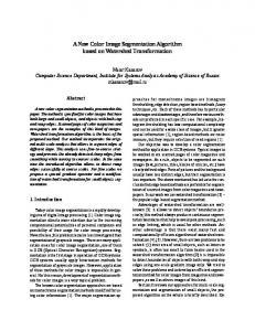
Fig. 1 (a) Grid Based Particle Method (GBPM) representation. (b) Determining the foot-point using a local least-square reconstruction of the interface.
ifold represented by unconnected sampling points in the GBPM formulation. Section 4 contains some experimental results. Finally, concluding remarks and discussion can be found in section 5.
2 Background 2.1 Convex Segmentation Models on Manifolds Total variation is a popular constraint in image segmentation because of its ability for removing small variations while smoothing boundaries between large segments. Many image segmentation methods have been proposed using TV regularization. For example, the well known Chan-Vese model [6] partitions an image using the piecewise constants approximation and TV regularization. However, the result from this model depends heavily on the choice of the initial guess. In order to overcome this difficulty, some interesting convex models and algorithms for K-phase image segmentation have been recently proposed in [10] (for K = 2) and [8,33]. The idea is to replace the typical indicator function u ∈ {0, 1} by a continuum version ∫ ∫ 2 E(u) = < (f − c) , u > dx + λ |∇u| dx, (1) Ω
Ω
where f : Ω → R is the given image intensity function, λ is a regularization parameter, and c = (c1 , c2 , · · · , cK )T contains the mean intensity in each phase. The relaxed classification function u : Ω → ∑K [0, 1]K is restricted on a convex set △+ = {u(x) : k=1 uk (x) = 1, 0 ⩽ uk (x) ⩽ 1}, where uk (x) is the k-th component of u. Since this cost functional is strictly convex, the model has a unique global minimizer and so the segmentation result does not depend on the choice of the initial parameters. This convex model has also been extended to manifolds recently in [17] ∫ ∫ E(u) = < (f − c)2 , u > dM + λ |∇M u| dM . (2) M
M
Here, the functions f and u are defined on a manifold M instead of a 2D Euclidean domain Ω, | · | is the Riemannian norm, ∇M is the intrinsic gradient defined on M and dM is the manifolds element measure. Numerically, such approach may be difficult since the regularization term in the energy has a singularity at 0, and the Euler-Lagrangian equation from the first order optimality is nonlinear and degraded. It is, therefore, numerically challenging to directly solve the partial differential equation on the manifold.
2.2 Grid Based Particle Method for Dynamic Interfaces For the convenience of readers, we give a brief summary of the Grid Based Particle Method (GBPM). For a complete and detailed description of the algorithm, we refer the readers to [1–4].
4
In the GBPM, we represent the interface by meshless particles which are associated to an underlying Eulerian mesh. Each sampling particle on the interface is chosen to be the closest point from each underlying grid point in a small neighborhood of the interface. This one to one correspondence gives each particle an Eulerian reference during the evolution. At the first step, we define an initial computational tube for active grid points and use their corresponding closest points as the sampling particles for the interface. A grid point y is called active if its distance to the interface is smaller than a given tube radius, ϵ, and we label the set containing all active grids Γ . To each of these active grid points, we associate the corresponding closest point on the interface, and denote this point by x. This particle is called the foot-point associated to this active grid point. Furthermore, we can also compute and store certain Lagrangian information of the interface at the foot-points, including normal, curvature and parametrization, which will be useful in various applications. This representation is illustrated in figure 1 (a) using a circular manifold as an example. We plot the underlying mesh in solid line, all active grids using small circles and their associated foot-points on the manifold using squares. To each grid point near the interface (blue circles), we associate a foot-point on the interface (red squares). The relationship of each of these pairs is shown by a solid line link. More importantly, associated to each of these footpoints and activated grid point, we also have a least square local approximation of the interface using polynomials in a local coordinate system, {(n)⊥ , n} with x as the origin, figure 1 (b). This will be very useful in solving partial differential equations (PDEs) on the interface [3, 4].
3 The Proposed Method 3.1 The New Splitting Methods on Manifolds To simplify the following expressions, we only consider the 2-phase segmentation, i.e. K = 2. Together with the convex relaxation range △+ , using the fact that u2 = 1 − u1 and rewriting u1 with u, then the cost functional (2) becomes ∫ ∫ ∫ E(u, c1 , c2 ) = (f − c1 )2 u dM + (f − c2 )2 (1 − u) dM + λ |∇M u| dM, (3) M
M
M
where 0 ⩽ u ⩽ 1. Instead of dealing with the energy directly, we propose to extend some recently developed operator splitting methods proposed in [34,12,14,11,13] which have been shown to be very efficient for solving L1 or total variation (TV) minimization problems in the 2-D plane image processing. In these algorithms, the singularity of L1 norm at 0 is transferred into a shrinkage problem together with a smooth minimization problem so that one can apply various stable and fast algorithms. Here, we employ the Augmented Lagrangian Method (ALM) (see e.g. [35]) to minimize the cost functional (3) on manifolds, which is an extension of ALM for TV [12] on 2D plane images. In order to overcome the non-smoothness of the L1 Riemannian norm, we have to separate the norm and the intrinsic gradient operator ∇M . The intrinsic gradient ∇M u is used to describe the variation of u on a manifold M. Suppose a surface (or a manifold) M is embedded into the Euclidean space R3 , then ∇M u is an orthogonal projection of the gradient vector ∇u in the embedding space onto M if u is well defined on entire R3 . Mathematically, the intrinsic gradient has the expression and has been implemented in the level set method framework [25] ( ) N⊗N < ∇u, N > N= I− ∇u, ∇M u = ∇u − |N|2 |N|2 where N is the normal vector on M, I stands for the 3 × 3 identity matrix, and the symbol ⊗ represents the Kronecker tensor product. In this paper, we do not intend to directly use this formulation of intrinsic gradient since it requires the gradient of u in the entire embedding space R3 which is not always available. On the other hand, if the manifold or surface M in 3D space has a parameterized expression x(s1 , s2 ), then the intrinsic gradient also can be written as [36] ∇M u =
( ∂x ∂s1
∂x ∂s2
( ) ( ∂u ) ) E F −1 ∂s 1 . ∂u F G ∂s2
5
Here E, F, G are the coefficients of the first fundamental form of surface M given by E =< ∂x ∂x ∂x ∂x F =< ∂s , >, G =< ∂s , >. As a result, one could obtain 1 ∂s2 2 ∂s2 |∇M u| =
√ (∇M u)T (∇M u) =
Now we let
√ ( ∂u ∂s1
∂x ∂x ∂s1 , ∂s1
)−1 ( ∂u ) √ ( )−1 ( ) EF ∂u ∂s1 T E F = (∇ u) ∇s u . s ∂u ∂s2 F G F G ∂s2
>,
(4)
( )−1 EF g := . F G
Introducing an auxiliary variable v, the variational problem (3) is equivalent to the following constrained optimization problem for ∇s u {∫ } ∫ ∫ √ 2 2 T (f − c1 ) u dM + (f − c2 ) (1 − u) dM + λ min v gv dM , u∈[0,1],v,c1 ,c2
M
M
M
such that v = ∇s u .
(5)
Since g is positive definite for regular surfaces, the condition v = ∇s u in (5) can be replaced by g(v − ∇s u) = 0. By applying a similar idea as in the ALM (see e.g. [35, 12]), the constraint problem (5) can be further rewritten as the following unconstraint Lagrangian functional for saddle point problem ∫ ∫ ∫ √ 2 2 L(u, v, p, c1 , c2 ) = (f − c1 ) u dM + (f − c2 ) (1 − u) dM + λ vT gv dM M M M ∫ ∫ η + < p, g(v − ∇s u) > dM + (v − ∇s u)T g(v − ∇s u) dM , (6) 2 M M where p is the Lagrangian multiplier, and η is a positive penalty parameter. Note however that such modification in (6) is not the classical ALM which should be given by ∫ η (v − ∇s u)T gT g(v − ∇s u) dM 2 M (such as [35, 12]). If one follows this original ALM directly, the sub-minimization problem for v would have no closed-form solution and it could slow down the convergence of the overall algorithm. On the other hand, our proposed modification in (6) would lead to a nice simple sub-minimization problem for v which can be solved easily using shrinkage. To numerically get a saddle point of L, we use the following alternating minimization algorithm n+1 n+1 n+1 n+1 ,v , c1 , c2 ) = arg min L(u, v, pn , c1 , c2 ) , (u
u∈[0,1],v,c1 ,c2
pn+1 = arg max L(un+1 , vn+1 , p, cn+1 , cn+1 ), 1 2 p
which can be further reduced into 4 subproblems: ˜ vn , pn , cn1 , cn2 ), un+1 = arg min L(u,
(7)
u∈[0,1]
˜ n+1 , v, pn , cn1 , cn2 ), vn+1 = arg min L(u
(8)
v
˜ n+1 , vn+1 , pn , c1 , c2 ), (cn+1 , cn+1 ) = arg min L(u 1 2
(9)
c1 ,c2
pn+1 = pn +
η g(vn+1 − ∇s un+1 ), Λmax
˜ is given by where Λmax is the maximum eigenvalue of matrix g and L ∫ ∫ ∫ √ ˜ v, p, c1 , c2 ) = L(u, (f − c1 )2 u dM + (f − c2 )2 (1 − u) dM + λ vT gv dM M∫ M M η 1 1 + (v − ∇s u + p)T g(v − ∇s u + p) dM . 2 M η η We can prove the following convergence of the above iteration:
(10)
6
Theorem 1 For any fixed u and c, the sequence (vn , pn ) produced by iteration (8) and (10) converges and vn → ∇s u. Proof 1 See Appendix A for details. Now, we only need to solve the above three minimization problems to update variables u, v, c1 and c2 . As to the subproblem (7), the associated Euler-Lagrange equation is the surface Laplace equation 2 2 2 2 √ ∑ ∑ ∑ ∑ η ∂ √ ∂u η ∂ 1 +√ EG − F 2 −√ EG − F 2 gij gij (vjn + pnj ) 2 ∂s ∂s η EG − F 2 i=1 ∂si EG − F j i j=1 i=1 j=1 2
2
+ (f − c1 ) − (f − c2 ) = 0, when u ∈ [0, 1] (11) where gij is the ij-th element of the matrix g, and the similar notations for vj and pj . The first term in the equation is the Laplace-Beltrami operator. We leave in Appendix B a detailed calculation in obtaining (11) from minimizing the subproblem (7). The subproblem (8) is a L1 − L2 minimization problem on manifolds which can be efficiently solved by the following g-shrinkage operator ( v
n+1
= shrinkg ∇s u
n+1
pn λ − , η η
) =
∇s un+1 − ||∇s un+1 −
pn η pn η ||g
) ( pn λ max ||∇s un+1 − ||g − , 0 , η η
(12)
√ where ||·||g is a weighted norm with the expression ||z||g = zT gz for any vector z. A detailed derivation of this g-shrinkage operator can be found in Appendix C. Indeed, there is another splitting scheme for this ˜Tg ˜ using, for example, the Cholesky decomposition, and introducing subproblem by decomposing g into g ˜ ∇s u. However, such formulation requires to differentiate g ˜ in the subproblem for u the condition v = g which is complicated. Finally, the means cn+1 and cn+1 can be easily updated with 1 2 ∫ ∫ n+1 fu dM f (1 − un+1 ) dM M M n+1 n+1 c1 = ∫ , c2 = ∫ . (13) n+1 n+1 u dM (1 − u ) dM M
M
To summarize, we get the following ALM for image segmentation on manifolds: Algorithm 1 Given initial guess values c01 , c02 . We set v0 = p0 = 0 and iterate the following steps until a convergence criterion is reached: Step 1: calculate un+1 by solving the PDE (11); Step 2: update vn+1 with the g-shrinkage operator (12); Step 3: determine the mean vector cn+1 according to (13); Step 4: find pn+1 using (10). There are several complications in the above algorithms. The first is that Steps 2 and 4 require computations of the surface gradient ∇s u on the manifold or surface which might be tricky depending on the manifold representation. The second is to solve the Laplace-Beltrami equation (11) in Step 1. The third is to compute integrals (13) in Step 3 on a general manifold. Indeed, these problems might be solved if we are given a surface triangulation. In this paper, however, we propose to apply and extend a newly developed GBPM proposed in [1–4] which provides another natural way to solve these subproblems. Details will be given in the next two subsections.
3.2 Computing Derivatives and Solving PDE on Manifolds in the GBPM Representation In this section, we explain how to incorporate the GBPM to compute derivatives of function and to solve a PDE on manifolds. These ideas will be similar to those proposed in [3, 4], but are slightly modified to better fit the current application. We will explain the difference in details in later paragraphs. The GBPM originally proposed in [1] is to model the interface motions. The key idea of GBPM is to sample the surface according to an underlying mesh such that each sampling particle is a L2 projection of the grid point in a neighborhood of the interface. Then the function and its derivative defined on
7
surface can be approximated in a local coordinate system, and thus we can solve various PDEs defined on an evolving interface represented by particles [3,4]. Assume that we are given a uniform Cartesian mesh in R3 which can well sample the manifold M. For each grid point yi near the manifold, we assume also that we are given its L2 projection onto the surface. We call this closest point the foot point and we denote it by xi = (xi1 , xi2 , xi3 )T . Further, we assume the image f is defined on these foot point locations, and we denote it by f i = f (xi ). These assumptions are mild comparing to other representations. For instance, we do not require the connectivity of these foot points as in the surface triangulation. Also, we do not require a specified normal vector at these foot points since it might not be available for non-orientable surface. Equivalent to this condition, which implies that we do not require a global implicit representation as in the level set function. Now, if the manifold M is smooth, it can be well-approximated by functions such as polynomials in a local coordinate system in a small local neighborhood of each xi . A detailed description of the construction is given here: 1. Determine the local neighborhood. For each neighboring grid point yi , we search m nearest activated grid point yj and collect their associated footpoints. We denote this set {xj }m j=1 . 2. Estimate the normal vector of the local coordinate system. We choose a unit direction n = (n1 , n2 , n3 )T in R3 which minimizes the sum of the squared differences of all the variation between xj and n. Mathematically, we minimize n = arg min |˜ n|=1
m ∑ (
˜ > − < xi , n ˜> < xj , n
)2
.
(14)
j=1
The minimizer of this problem can be determined by finding the eigenvector corresponding to the )( )T ∑m ( smallest eigenvalue of the symmetry matrix H = j=1 xj − xi xj − xi . A simple proof is given in Appendix D for completeness. Further, if xi is the mean of all the xj (which is not the case in the current application), (14) is equivalent to the well known principal component analysis (PCA). 3. Construct a coordinate system with the three eigenvectors T1 , T2 , n of H as the x-axis, y-axis and z-axis respectively. We denote this coordinate system as {xi ; T1 , T2 , n}. Once we obtain the local coordinate system, we can easily approximate the metric tensor of manifold and the derivatives of any function defined on this manifold. In particular, let us assume that the manifold or the surface in a local neighborhood is approximated by a degree k polynomial. For each xj , ¯ j be the new coordinates of xj in the local system {xi ; T1 , T2 , n}, i.e. j = 1, · · · , m, let x 2 n1 n1 n2 n1 ( 1+n3 − 1 1+n3 ) j i n22 ¯ j = n1 n2 x − 1 n2 x − x . 1+n3
n1
1+n3
n2
n3
Now, assume the underlying manifold is locally quadratic, i.e. x ¯3 (¯ x1 , x ¯2 ) ≈
2 ∑
∑
ατ1 τ2 x ¯τ11 x ¯τ22 ,
τ1 =0 0⩽τ1 +τ2 ⩽2
in which ατ1 τ2 are some unknown coefficients. For every activated grid point yi near the manifold, these local coefficients ατi 1 τ2 can be determined by minimizing the following least squares sum: 2 m 2 ( )τ1 ( )τ2 ∑ ∑ ∑ j j j x ¯3 − ατi 1 τ2 x ¯1 x ¯2 . j=1
Denote
τ1 =0 0⩽τ1 +τ2 ⩽2
( i ) i i i i i T α01 α02 α10 α11 α20 αi = α00 , 1 x ¯12 (¯ x12 )2 x ¯11 x ¯11 x ¯12 (¯ x11 )2 2 1 x x22 )2 x ¯21 x ¯21 x ¯22 (¯ x21 )2 ¯2 (¯ A = . . , .. .. .. .. .. .. . . . . 2 m m m 2 1x ¯m xm ¯1 x ¯1 x ¯2 (¯ xm 2 (¯ 2 ) x 1 ) m×6 ( 1 2 ) T ¯3 x ¯3 · · · x ¯m b= x , 3
then this least square polynomial can be obtained by solving the over-determined linear system Aαi = b,
8
by the SVD or the QR decomposition. As a result, the elements of metric tensor E i , Gi , F i at xi occur in equation (11) can be approximated using E i =< Gi =< F i =
=< > =< > =
≈ 1 + (α10 + α11 x ¯i2 + 2α20 x ¯i1 )2 , i i i > ≈ 1 + (α01 + α11 x ¯i1 + 2α02 x ¯i2 )2 , i i i i i i i i > ≈ (α10 + α11 x ¯2 + 2α20 x ¯1 )(α01 + α11 x ¯i1 + 2α02 x ¯i2 ).
Similarly, the relaxed classification function u defined on the manifold can be approximated using least squares approximation [3,4] u(¯ x) ≈
2 ∑
∑
βτ1 τ2 x ¯τ11 x ¯τ22 .
τ1 =0 0⩽τ1 +τ2 ⩽2
Mathematically, we need to solve the least square fitting problem with energy 2 m 2 ( )τ1 ( )τ2 ∑ ∑ ∑ u(¯ xj ) − βτi τ x ¯j1 x ¯j2 . 1 2
τ1 =0 0 ϵ δϵ (ϕ) = πϕ 1 1 , |ϕ| ≤ ϵ 2ϵ + 2ϵ cos ϵ for ϵ = 1.5∆y. For a more detailed analysis of the approximation, we refer interested readers to [38, 39]. To approximate (17) in the current application, we first convert the GBPM representation to the level set representation within ϵ-distance from the interface, i.e. we will activate any grid point which has distance from it’s foot point less than ϵ = 1.5∆y. This is simple in the GBPM since the foot point xi is defined to be the L2 projection of the activated grid point yi onto the interface M, which means the distance function |ϕi | = ∥xi − yi ∥2 . Next, the level set formulation (17) requires an extension of f from M to Ω, at least in the ϵ-neighborhood of M. A natural way to do is the orthogonal extension. Once again, since xi is the L2 projection of yi onto M, we simply use f (yi ) = f (xi ). To conclusion, we approximate the surface integral (17) using ∫ ∑ f (s)ds ≃ f (yi ) δϵ (∥xi − yi ∥2 )∆y . (18) M
i
If we let ϵ in delta function δϵ be very small (less than 0.5∆y), then the discrete formulation (18) for integration calculation only to sum up the points defined on the manifold. This means that we do not need the signed distance function in practice. We shall use this fact to update ci when the surface is open. After we finished this work, an integration computation method for the point cloud representation is proposed in [40] by using local mesh method, thus our segmentation algorithm also can be implemented on the point cloud data by combining with their method.
4 The Experimental Results In this section, we show the image segmentation results on various of 2-D manifolds with the proposed algorithm. All these manifolds are represented by GPBM and the images defined on these manifolds contain noise. In all the experiments, the image intensity f are normalized in [0, 1], and the initial means c01 , c02 are set as 0.33, 0.66 respectively. In addition, the classification functions u are often segmented into a binary image using a simple threshold at the value 0.5.
10
4.1 Segmentation on Closed Geometric Surfaces First, we test our method on some closed geometric surfaces. Fig.2 shows some segmentation results with algorithm 1 on a sphere. In this figure, several simple geometry objects are mapped onto a sphere surface. The foot points xi are given by ||xi − 0.5||22 = 0.42 (a sphere centered at (0.5,0.5,0.5), with radius 0.4) on domain [0, 1] × [0, 1] × [0, 1], while the underlying computation mesh grid size is 200 × 200 × 200. The intensities on the sphere are piecewise constants and corrupted by noise with a standard deviation 100 255 . In the experiments, the regularization parameter λ is set to 2.0 × 10⁻⁵ and the penalty parameter is fixed as 10λ. In order to better show the visual effect of the segmentation, three images from different views are given in Fig.2 (a)-(c), respectively. In the second row of this figure, the corresponding segmentation results are displayed. In these figures, we use different colors to represent different classes. It can be seen that the proposed algorithm can provide good results in this situation: the line on the sphere are straight along with the sphere and the curves are smooth though there are heavy noise in the original images. To compare the segmentation without regularization, the results with k-mean (i.e. set regularization parameter λ as 0) are illustrated in the third row of Fig.2. Fig.3 shows some classification results for the noisy world map on the earth. It can be seen that the proposed method can well segment this map. Segmentation result on a smooth torus is displayed in Fig.4. In this experiment, a brain MR image is mapped onto a cloud points based torus, then the proposed algorithm is applied to segment the torus into 2 parts. Fig.4 (b) shows the final classification result. In this figure, we still use different color to represent the different classes.
4.2 Segmentation on Open Geometric Surfaces Since the PDE is directly solved on particles (foot points) in the proposed method, it works well on the open surfaces, which may be difficult for implicit methods such as the level set method. Fig.5 shows that the proposed method nicely segments the cameraman image on a cylindrical surface into 2 parts. To test more complicated surfaces, we applied the proposed algorithm on a Mobius strip which is open and is not orientable, and thus it has no level set representation. We have tested two different images on the strip and the results are shown in Fig.6 (b) and (d), respectively. In order to show the details of the GBPM surface, we zoom-in to these solutions and plot the results in Fig.6 (e) and (f). Note that the colors in these figures do not correspond to the true intensity value of the binary label function u, but is only used to represent the two different classes.
4.3 Segmentation on Some Scanned Surfaces in Applications We test the proposed algorithm on the scanned Stanford bunny data (http://graphics.stanford. edu/data/3Dscanrep/ ). We define a piecewise image f on the bunny with noise (see the figures in the first row of Fig.7). The level of the noise is high, with a standard derivation 100 255 . We have shown our segmentation results in Fig.7 (d)-(f). To better show our results, we zoom-in to these solutions and plot our solutions in Fig.7 (g) and (h), respectively.
5 Discussions and Conclusions We propose a method to segment images defined on manifolds represented by the GBPM. This method extends the convex segmentation methods on 2-D plane images to some general manifolds. By integrating the recently developed operator splitting techniques, we use some local approximation methods to solve the PDE which comes from the energy minimization on the foot points. Compared to the level set method, our proposed method provides a flexibly representation to handle open manifolds which are difficult to be defined using a signed distance function. In this paper, even though we have only discussed the 2 phases segmentation, one can easily extend the method to address the multi-phases clustering. The proposed method can be further improved by employing the adaptive mesh techniques and some other local fitting techniques. It can also be extended to some other image processing areas such as image registration and restoration.
11
(a)
(b)
(c)
(d)
(e)
(f)
(g)
(h)
(i)
Fig. 2 (a-c) The noisy image on a sphere with 3 different views (using MATLAB function view(75,30), view(-15,-45) and view(-70,30), respectively). (d-f) Segmentation results using the proposed algorithm. (g-h) Segmentation results without the regularization term.
Acknowledgement Leung would like to thank Prof. Ronald LM Lui for providing a conformal map of the Stanford bunny data to a sphere. The work of Leung was supported in part by the Hong Kong RGC under Grant DAG09/10.SC02 and the HKUST grant RPC11SC06. The work of Liu was supported by National Natural Science Foundation of China (No. 11201032).
Appendix A. Proof of Theorem 1 We first prove the following lemma Lemma 1 Suppose J1 (v) is continuous and convex on a Hilbert space V, and J = J1 (v)+ < p, g(v − b) > +
η < v − b, g(v − b) > 2
12
(a)
(b)
(c)
(d)
(e)
(f)
Fig. 3 (a,c,e) The world map on a sphere using 3 different views. (b,d,f) Our segmentation results.
(a)
(b)
Fig. 4 (a) Brain image on torus. (b) Our segmentation result.
where η > 0 and g is a positive definite and linear symmetric operator with bounded inverse, then the sequence {vn } produced by the iteration scheme vn+1 =arg min J (v, pn ),
(19)
pn+1 =pn + τ g(vn+1 − b),
(20)
v
13
(a)
(b)
Fig. 5 (a) The mapped cameraman image on the cylinder. (b) Our segmentation results.
(a)
(b)
(c)
(d)
(e)
(f)
Fig. 6 (a,c) Noisy images mapped on the Mobius strip. (b,d) Our segmentation results. (e,f) Zoom-in of (a) and (b), respectively.
converges, i.e. vn → v∗ when 0 < τ < Λmax is the largest eigenvalue of g.
2η Λmax ,
where v∗ is the saddle point (v∗ , p∗ ) of J (v, p) . Here
14
(a)
(b)
(c)
(d)
(e)
(f)
(g)
(h)
Fig. 7 Segmentation on the Stanford bunny data by our method. (a-c) The noisy images on the bunny. (d-f) Our segmentation results. (g-h) Zoom-in of the results in (d-f). ∗ ∗ Proof Since (v∗ , p∗ ) is a saddle of J , then we have v∗ = b by ∂J ∂p |(p ,v ) = 0. Let ∂J1 (v) is the ¯ ¯ is the ¯ , q − v >, ∀q ∈ V}, where V subgradient of J1 at v, i.e. ∂J1 (v) = {¯ v ∈ V : J1 (q) − J1 (v) ⩾< v conjugate space of V. According to the first order optimization conditions of (19), we have
dn+1 := −gpn − ηg(vn+1 − b) ∈ ∂J1 (vn+1 ), d∗ := −gp∗ − ηg(v∗ − b) ∈ ∂J1 (v∗ ), thus
dn+1 − d∗ = −g(pn − p∗ ) − ηg(vn+1 − v∗ ).
Taking inner product with vn+1 − v∗ for both sides of the above equation, it becomes < pn − p∗ , g(vn+1 − v∗ ) >= − < dn+1 − d∗ , vn+1 − v∗ > −η < vn+1 − v∗ , g(vn+1 − v∗ ) > . By the iteration equation (20) and the fact that v∗ − b = 0, we have pn+1 − p∗ = pn − p∗ + τ g(vn+1 − v∗ ).
(21)
15
Taking norm for the both sides of the above equation, we get ||pn+1 − p∗ ||2 = ||pn − p∗ ||2 + τ 2 ||g(vn+1 − v∗ )||2 + 2τ < pn − p∗ , g(vn+1 − v∗ ) > .
(22)
Substituting (21) into (22), we have ( ) ||pn+1 −p∗ ||2 −||pn −p∗ ||2 = −2τ < dn+1 −d∗ , vn+1 −v∗ > − < vn+1 −v∗ , −τ 2 g2 + 2τ ηg (vn+1 −v∗ ) > . (23) Since J1 is convex, dn+1 ∈ ∂J1 (vn+1 ) and d∗ ∈ ∂J1 (v∗ ), thus < dn+1 − d∗ , vn+1 − v∗ >⩾ 0.
(24)
With the condition 0 < τ < Λ2η , we can conclude that the operator −τ 2 g2 + 2τ ηg is positive definite. max Now, using both (23) and (24), we have ||pn+1 − p∗ ||2 − ||pn − p∗ ||2 < 0, which implies that the sequence ||pn − p∗ ||2 is monotonic decreasing with a lower bound 0 and so it must be convergent. Finally from (23), we conclude that vn → v∗ . ∫ √ Now, we can use this Lemma to proof Theorem 1. It is easy to check that λ M vT gv dM is convex when g is positive defined. For any fixed u and c, let b = ∇s u and following the lemma, one can get that {vn } produced by equations (8) and (10) converges to the saddle point (·, v∗ , p∗ , ·) of L(·, v, p, ·), i.e. vn → v∗ . Since (·, v∗ , p∗ , ·) is the saddle point, and we get v∗ = ∇s u, which completes the proof. Appendix B. Derivation of (11) The directional derivative {∫ ∫ ˜ + τ w) dL(u d |τ =0 = (f − c1 )2 (u + τ w) dM + (f − c2 )2 [1 − (u + τ w)] dM dτ dτ ∫ M M } 1 T 1 η (v − ∇s (u + τ w) + p) g(v − ∇s (u + τ w) + p) dM |τ =0 + 2 {∫ η η M } √ η d 1 T 1 2 = EG − F (v − ∇s (u + τ w) + p) g(v − ∇s (u + τ w) + p) ds |τ =0 2 ∫dτ η η ∫ [ ] 2 2 + (f − c1 ) − (f − c2 ) w dM M ∫ ∫ √ [ ] 1 EG − F 2 < gv − g∇s u + gp, ∇s w > ds + (f − c1 )2 − (f − c2 )2 w dM = −η η ) ∫ ∫ (√ ∫ M [ ] 1 = η ∇s · EG − F 2 (gv − g∇s u + gp) w ds + (f − c1 )2 − (f − c2 )2 w dM η M) (√ ∫∫ 1 1 2 √ =η ∇s · EG − F (gv − g∇s u + gp) w dM 2 η ∫M EG − F [ ] + (f − c1 )2 − (f − c2 )2 w dM. M
By the variational formulation
˜ ˜ + τ w) δL dL(u |τ =0 =< , w >, one gets dτ δu
(√ ) (√ ) ˜ δL η η 1 = −√ ∇s · EG − F 2 g∇s u + √ ∇s · EG − F 2 g(v + p) δu η EG − F 2 EG − F 2 2 2 +(f − c1 ) − (f − c2 ) , which leads to equation (11).
Appendix C. Derivation of (12) Denote qn = ∇s un+1 −
pn η ,
we have ˜ δL λ =√ gv + ηg(v − qn ). T δv v gv
16
Solving
˜ δL δv
= 0 for v, we get λ (√ + η)vn+1 = ηqn . n+1 (v )T gvn+1
(25)
Taking modulus || · ||g for the two sides of (25), it becomes ||vn+1 ||g = ||qn ||g −
λ η
if ||qn ||g ⩾ λη . Plugging it back to the above (25), we get vn+1 =
qn λ (||qn ||g − ). n ||q ||g η
(26)
On the other hand, if ||qn ||g < λη , then ∫
∫ √ η vT gv dM + (v − q)T g(v − qn ) dM 2 ∫M √ ∫M ∫ η vT gv dM + (||v||2g + ||qn ||2g ) dM − η vT gqn dM =λ 2 ∫M √ ∫M ∫M η ⩾λ vT gv dM + (||v||2g + ||qn ||2g ) dM − η ||v||g · ||qn ||g dM 2 M M M ∫ η (||v||2g + ||qn ||2g ) dM. > 2 M
˜ L(v, ·) = λ
˜ with respect to v. Summarizing these two results, This means that vn+1 = 0 must be the minimizer of L we get the g-shrinkage operator (12).
Appendix D. Minimizer of (14) λ1 ) ( ) ∑m ( j T Let H = j=1 x − xi xj − xi = U λ2
( ) UT , where λ1 ⩾ λ2 ⩾ λ3 and U = U1 U2 U3 is λ3
an orthogonal matrix. Then λ1 ) ( ) ∑m ( 2 T E = j=1 < xj , n ˜ > − < xi , n ˜> =n ˜ T H˜ n = UT n ˜ λ2
( ) UT n ˜ . λ3
( )T ( T ) Since UT n ˜ U n ˜ = 1, thus we have E ⩾ λ3 . If n ˜ = U3 , E = U3T HU3 = λ3 . Thus we conclude that n = U3 is a minimizer of E such that |n| = 1, which completes the proof.
Appendix E. Explicit formula for the gradient descent update ∆ui In this Appendix, we state explicitly the formula to compute the gradient descent update of ui as a function of the coefficients of the second order polynomial approximation in the GBPM representation. For convenience, let us denote hj = vjn + η1 pnj and write the coefficients of the approximated second-degree polynomial at xi for functions h1 and h2 as γτi 1 τ2 , δτi 1 τ2 (0 ⩽ τ1 + τ2 ⩽ 2, τ1 , τ2 ∈ N), respectively. The PDE (11) in the explicit form is given by [ ] η 1 η (S1 + S2 S3 + S4 S5 ) + S6 + S7 + S8 + S9 + (f − c1 )2 − (f − c2 )2 = 0 , − EG − F 2 EG − F 2 EG − F 2
17
where ∂2u ∂2u ∂2u − 2F +E 2 , 2 ∂s1 ∂s1 ∂s2 ∂s2 2 ∂ x ∂x ∂ 2 x ∂x 1 =< , >−< , >− (T1 G − T2 F ) , ∂s1 ∂s2 ∂s2 ∂s22 ∂s1 EG − F 2 ∂u , = ∂s1 ∂2x ∂x ∂ 2 x ∂x 1 , >−< , >− (T2 E − T1 F ) , =< 2 ∂s1 ∂s2 ∂s1 ∂s1 ∂s2 EG − F 2 ∂u = , ∂s2 ) ( ∂x ∂ 2 x ∂x ∂2x , >−< , > , = h1 < ∂s1 ∂s2 ∂s2 ∂s22 ∂s1 ( ) ∂2x ∂x ∂ 2 x ∂x = h2 < , >−< , > , ∂s1 ∂s2 ∂s1 ∂s21 ∂s2 ( ) ∂h1 ∂h2 ∂h1 ∂h2 =G −F + +E , ∂s1 ∂s1 ∂s2 ∂s2 = (Gh1 − F h2 ) T1 + (−F h1 + Eh2 ) T2
S1 = G S2 S3 S4 S5 S6 S7 S8 S9 and
( ) ∂ 2 x ∂x ∂2x ∂x ∂ 2 x ∂x ∂2x ∂x , , > G+ < , > E − < > + < , > F, ∂s21 ∂s1 ∂s1 ∂s2 ∂s2 ∂s21 ∂s2 ∂s1 ∂s2 ∂s1 ( ) ∂2x ∂x ∂ 2 x ∂x ∂2x ∂x ∂ 2 x ∂x T2 = < , , , > G+ < > E − < , > + < > F. ∂s1 ∂s2 ∂s1 ∂s22 ∂s2 ∂s1 ∂s2 ∂s2 ∂s22 ∂s1 T1 =