Search Image Segmentation Algorithm for Mine-like

-Search Image Segmentation Algorithm for Mine-like Objects Segmentation in SONAR Images Ivan Aleksi*, Benjamin Lehmann**, Tai Fei***, Dieter Kraus***, Željko Hocenski* *

**

Faculty of Electrical Engineering, University of Osijek, HR-31000 Osijek, Croatia. ATLAS ELEKTRONIK GmbH, Sebaldsbrücker Heerstrasse 235, D-28309 Bremen, Germany. *** Hochschule Bremen, University of Applied Sciences, Institute of Water-Acoustics, Sonar-Engineering and Signal-Theory, D-28199 Bremen, Germany.

[email protected], [email protected], [email protected], [email protected] Abstract: This paper addresses a SONAR image segmentation method employing a novel -Search Image Segmentation (ASSIS) algorithm. ASSIS is applied on Mine-Like Objects (MLO) in SONAR images, where an object is defined by highlight and shadow regions, i.e. regions of high and low pixel intensities in a SONAR image. Usually, the Search is used in mobile robotics for finding the shortest path, where the environment map is predefined and the start/goal locations are known. The ASSIS algorithm represents the image segmentation problem as a path-finding problem. Main modification concerning the original Search is in the cost function that takes pixel intensities in order to navigate the 2D segmentation contour. Firstly, the ASSIS algorithm uses a pixel intensity thresholding technique to build a goal distance map with the numerical navigation function (NNF). The NNF uses the L2 norm to estimate the Euclidean distance between the current pixel and a goal pixel. The estimated distance is then recalculated as predicted cost to the goal. So far made cost is calculated according to the current path length. Finally, the sum of and defines the cost function that determines the next contour point around an MLO. Keywords:

I.

-Search, Image Segmentation, Path Finding

INTRODUCTION AND RELATED WORK

Image segmentation plays an important role in image processing, and with the development of computers it became usable in many practical applications like medical imaging, machine vision for recognizing faces, iris and fingerprints, etc. However, it enables the selection of specific objects in an input image such that a human can more easily detect isolated areas of interest. Usually, image segmentation is used in autonomous systems, where the human interaction is replaced by machine vision. After the Second World War, underwater mines possess a real threat to the human population by endangering missions that include ships, submarines, etc. There are several types of anti-ship and -submarine mines (moored, limpet, contact, manta, cylinder, etc.) that are usually recognized by acoustic vision systems. Subsequently, they are usually destroyed with remotely operated vehicles (ROV), which are controlled by man, or with autonomous underwater vehicles (AUV). Mine-like Object (MLO) detection missions are usually done with a Side-scan SONAR systems [1]. After inspection of a certain area, a huge SONAR image is recorded. It has to be filtered to select smaller images, the socalled regions of interest (ROI). Effective ROI selection is done in [2]. Each ROI is then used as an input image to the segmentation process.

II.

ASSIS:

-SEARCH IMAGE SEGMENTATION

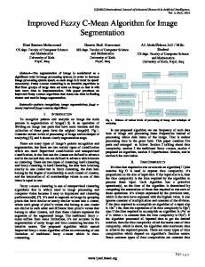
Usually, the -Search is used in conjunction with numerical navigation function for navigation in mobile robotics [3]. However, the application of the well-known -Search to image segmentation in general, as well as MLO segmentation in SONAR images, is a novel practical application, at least to our knowledge. -Search Image Segmentation (ASSIS) algorithm uses the basic Search method with a modified cost function. ASSIS divides an original gray scale ROI image into two parts, by inserting an artificial wall, c.f. Fig. 1a, that enables path plans for both parts independently, c.f. Fig. 1b. Start and goal positions are assigned at the beginning and the end of the detected object/shadow region. A. Object and Shadow Region Input image is relatively small size ROI image with detected MLO that typically has highlight (object) and shadow (dark) regions, as it is illustrated in Fig. 1a and Fig. 2a. Threshold technique is used to determine highlight region if a pixel intensity is above , and shadow region if a pixel intensity is below . As it is illustrated in Fig. 1a, pixel intensities that are colored with gray are the values above and below . They are considered as restricted obstacle regions that planner avoids by planning around them. Threshold results for highlight and shadow regions are depicted in Fig. 2b and 2c, respectively.

Figure 1. Region of interest in 8-bit grayscale SONAR image with Mine-like object and: (a) thresholded pixel intensity levels; (b) inserted artificial wall that divides object/shadow region into two parts and enables mapping of a path-planning process as a segmentation process.

B. Numerical Navigation Function Numerical navigation function (NNF) is a potential field-based navigation function (terrain information is also used in the literature). Firstly it was defined for wheeled mobile robot trajectory planning strategies [4]. Those methods interact with robot as with a ball in a configuration space affected by an imaginary potential field. This potential field pushes a robot away from collision with obstacles (obstacle region) in robot’s environment, while it pulls a robot into a goal configuration. Analytic construction of navigation function over free region (nonobstacle region) of arbitrary geometry is in general a complex task. However, if free region is represented with grid of cells, numerical navigation function (NNF) can be very efficient with integer programming implementation [5]. In this work, the NNF value is assigned to each pixel of the input image that is below the threshold value (above ), c.f. Fig. 1a. Pixels with values above (below ) value are considered as obstacles and they do not have the NNF value assigned. NNF value is calculated based on eight neighbor pixels NNF values. In order to calculate NNF value for neighbor pixels , where , following equations are used. (1) (2)

C. Path Planning Algorithm: -Search Let graph be an undirected graph, where is a vertex set and is an edge set. Vertex is connected with vertex if there is an edge between and . Vertex represents the robot configuration defined with (3) where stands for the observed pixel and is the angle calculated from current pixel to the neighbor pixel . Let be a tree structure with vertex as its root. Root vertex is inserted in with the ROOT function. Tree consists of visited vertices . Each visited vertex is connected in with its corresponding parent vertex . This connection in is done with a function CONNECT and is also denoted with . Let be the list of vertices sorted according to their cost function value , which is calculated as follows (4) where is a number of vertices from vertex to current vertex in a solution tree , is the NNF value assigned to the current vertex . So-far made cost is , while stands for estimated cost to the goal. The following functions are used to manipulate with the list . Function INSERT inserts vertex into the list that is sorted according to the vertex cost function value (4). Initial vertex is inserted with the zero cost.

Figure 2. Region of Interest (ROI), 8-bit resolution, image with detected Mine-Like Object (MLO) (a); assigned maximum pixel intensity values for pixels with intensities above threshold for object (b) and shadow region (c). Assigned Numerical Navigation Function (NNF) values to each pixel, for object (d) and shadow region (e), respectively, with added artificial wall that enables path planning around the MLO. Colorbar (a) is also valid for (b), (c), (d) and (e) images. Red pixel denotes obstacle regions with simply 255 intensity value that path planner avoids by planning a path around them.

Function EMPTY returns TRUE if the list is empty, otherwise FALSE. Function SORT sorts the list by ascending cost function value. Function FIRST returns a first vertex from the sorted list and deletes the same vertex in . Function GOAL returns TRUE if a goal vertex is reached, otherwise FALSE. Goal is reached when a vertex has position equal to the goal pixel that is input to (Alg.1). Function VISITED tests, while function MARK_VISITED marks vertex (3) as visited in order to avoid repeated search at the same location. -Search algorithm (Alg.1) input parameters are: graph , the NNF matrix , initial vertex and a goal vertex . Output parameter is the tree that contains segmented path around MLO that connects pixel with pixel . -Search algorithm begins with the empty list and the empty tree , with initially inserted

Algorithm 1.

Input: Output: 1: 2: 3: 4: 5: 6: 7: 8: 9: 10: 11: 12: 13: 14:

-Search algorithm.

as a path from

to

Create empty list and tree INSERT ROOT while not EMPTY do SORT set FIRST if GOAL then return as the solution. if not VISITED set EXPAND for each vertex in MARK_VISITED CONNECT INSERT return solution not found.

starting vertex in both of them (Alg.1 lines 1-3). While is not empty list (Alg.1 lines 4-12), is sorted and the vertex with smallest cost function value is taken from (Alg.1 lines 5-6). If goal vertex is reached, the algorithm returns the tree as the solution (Alg.1 line 7). Since goal vertex is not reached, vertex is tested if it was visited already, by a function VISITED (Alg.1 line 8). If a vertex is not visited, the algorithm will search for vertices that are connected with . Vertices are marked as visited by setting a flag in a binary 3D matrix, that consists of 2D positions and 1D orientations (3). The EXPAND function returns set of vertices that are connected with (Alg.1 line 9). Vertices that are connected with current vertex are inserted into and (Alg.1 lines 11-13). As a result, the tree consists of expanded vertices in , i.e. it contains edges and vertices that connects a goal vertex with the root vertex . Finally, a path is reconstructed by following edges in , backwards, from a goal vertex to a start vertex . Edges of a graph define a set of connected vertices, i.e. edges. Set consists of visited vertices that are connected with their parent vertex . Set is calculated from ROI image pixels and orientation (3). Parent vertex corresponds to the currently observing pixel in the ROI image. Visited vertices correspond to pixels in the ROI image that are neighbor pixels of . Determining connections between and is also denoted with expanding vertex . Geometrical constraints that define neighbor pixels , i.e. visited vertices , are the distance (5) and maximum angle change (6). Pixel intensity constraint additionally reduces the number of vertices in . Vertices are remaining in the set if their assigned pixel intensity value is below threshold for the highlight region (7) and above threshold for the shadow region. Additionally, vertex is removed from the set if (8) is not satisfied, i.e. if any of pixels that are on the line between and have pixel intensity above threshold . Finally, eq. (5-7) define the set of vertices that are connected with parent vertex .

Figure 3. Set of visited vertices are connected with their parent vertex

(corresponds to pixel that (corresponds to pixel ).

(5) (6) (7) (8) Equations (5-6) are maximum distance and angle constraints, respectively, c.f. Fig. 3. Pixel intensity constraints (7-8) compare ROI image pixel intensities with threshold value for the highlight region. For the shadow region, equality is used in (7) and (8), with threshold value . D. ASSIS method In this paper, segmentation of MLO's is applied on the input 8-bit ROI image with width , height and pixel intensity values ranging from 0 to 255. Selection of smaller ROI images from larger SONAR images is proposed in [2]. In order to align a SONAR scanning direction, ROI images considered in this paper are rotated so that the SONAR scanning direction is from the bottom to the top. Therefore, highlight regions appear before the shadow regions. Before using the NNF and the -Search methods, the obstacle regions and the free regions are calculated. Firstly, the artificial wall placements are done by placing lines , as it is illustrated horizontally in Fig. 1a and vertically in Fig. 2d and 2e. ASSIS method uses lines and places them vertically with distance apart (9). Subsequently, a start position and a goal position are calculated along in order to plan a path between start and goal positions. Start position is determined as the first value above threshold (below ). Goal pixel is determined by its square neighborhood, defined by number of pixels to the left, right and forward direction along line . Total number of goal neighbor pixels is defined with (10). Finally, goal pixel is set to the pixel if at least 90% of its neighbor pixels are located in the free region (11). (9)

(10) (11) After defining a line , a start position and a goal position , four copies of input image are created, , , and and are used to define the obstacle and the free region for the highlight and shadow, and for the left and right segmented contours, respectively. For highlight images and , pixel intensities above are set to 255. For shadow region images and , pixel intensities below are set to 255. Obstacle region is defined with maximum pixel intensity value 255, while free region is defined with pixel intensities from 0 to 254. Path planner uses only free region to plan a segmented path around MLO. Subsequently, artificial wall is placed in ( ) by 1 pixel to the left from the line in order to calculate right segment of a contour around MLO's highlight (shadow). Analogously, artificial wall is placed in ( ) by 1 pixel to the right from the line in order to calculate left segment of a contour around MLO's highlight (shadow). With created images , , and , the NNF and the -Search methods are executed four times, twice for highlight region and twice for shadow region. Resulting left and right planned paths are connected into a single path for a highlight region and for a shadow region . Finally, the highlight region contour and the shadow region contour denote the segmented MLO's highlight and shadow regions, respectively. Additionally contours (polygons) with relatively small surfaces and short lengths are removed from results. III.

EXPERIMENTAL RESULTS

Experimental results are done with four input ROI images, c.f. Fig. 4a, d, g, j. Parameters used for proposed ASSIS method are listed in Tab. 1. Resulting contours and are calculated with 20 vertically placed lines L distanced apart by . Resulting contours are displayed with red and green colored lines, for highlight and shadow, respectively, c.f. Fig. 4b, e, h, k. Finally, segmentation results are illustrated in Fig. 4c, f, i, l, with green colored background, blue colored shadow and red colored highlight region. Table 1. Input parameters in pixel intensity values and pixel number. 81 50 50 50

106 100 100 100

135 100 120 100

2 2 2 2

3 2 2 2

5 5 5 5

48 48 48 48

(c)

(d)

(e)

(f)

(g)

(h)

(i)

segmentation was done with no false detection. However in the third image, segmentation resulted with broadened shadow region and single misdetection in shadow region. Reason for misdetection comes from rough thresholding technique that depends on the measurement itself and has to be adjusted manually. On the other hand, determining start and goal positions in a more suitable way can significantly improve the ASSIS method segmentation results. REFERENCES

4 4 4 4

160° 160° 160° 160°

Experiment was done on a standard PC with i5 CPU. For image of size 81 x 106 pixels, the ASSIS method execution time in MATLAB is on average 3 s per line . IV.

(b)

(j) (k) (l) Figure 4. Input Region Of Interest (ROI) images (a, d, h, j ); calculated contours (light red colored lines) and (light green colored lines) using proposed -Search Image Segmentation (ASSIS) method (b, e, h, k ); and segmentation results with background (green), shadow (blue) and highlight (red) regions (c, f, i, l ). Images are in jet color map.

0.9·

Image

(a)

DISCUSSION AND CONCLUSION

Segmentation results, c.f. Fig. 4, illustrate that proposed ASSIS method segments MLO in ROI image in an appropriate way. In first two images, and in fourth image,

[1] [2]

[3]

[4] [5]

Blondel, P.: The Handbook of Sidescan Sonar. // Praxis Publishing Ltd, Chichester, UK, 2009. ISBN: 978-3-540-42641-7. Lehmann, B.; Siantidis, K.; Aleksi, I.; Kraus, D.: Efficient presegmentation algorithm for sidescan-sonar images. // Image and Signal Processing and Analysis (ISPA), 2011 7th International Symposium on, pp.471-475, 4-6 Sept. 2011. Cupec, R.; Aleksi, I.; Schmidt, G.: Step sequence planning for a biped robot by means of a cylindrical shape model and a highresolution 2.5D map. // Robotics and Autonomous Systems, Vol. 59, No. 2, pp. 84-100, February 2011. J. C. Latombe: Robot Motion Planing. // Kluwer Academic Publishers, Norwell, Massachusetts, USA, 1991. R. Cupec, G. Schmidt: An Approach to Environment Modeling for Biped Walking Robots. // International Conference on Intelligent Robots and Systems, 2005.