A stable and optimized neural network model for ...

Zeng & Huang

A stable and optimized neural network model for crash injury severity prediction

Qiang Zeng, Ph.D. Candidate Urban Transport Research Center, School of Traffic and Transportation Engineering, Central South University, Changsha, Hunan, 410075 P.R. China Email: [email protected]

Helai Huang, Ph.D., Professor* Urban Transport Research Center, School of Traffic and Transportation Engineering, Central South University, Changsha, Hunan, 410075 P.R. China Tel: 86 731 82656631 Email: [email protected]

* Corresponding author

Submitted for publication in Accident Analysis & Prevention August 13, 2014

1

Zeng & Huang

2

ABSTRACT The study proposes a convex combination (CC) algorithm to fast and stably train a neural network (NN) model for crash injury severity prediction, and a modified NN pruning for function approximation (N2PFA) algorithm to optimize the network structure. To demonstrate the proposed approaches and to compare them with the NN trained by traditional back-propagation (BP) algorithm and an ordered logit (OL) model, a two-vehicle crash dataset in 2006 provided by the Florida Department of Highway Safety and Motor Vehicles (DHSMV) was employed. According to the results, the CC algorithm outperforms the BP algorithm both in convergence ability and training speed. Compared with a fully connected NN, the optimized NN contains much less network nodes and achieves comparable classification accuracy. Both of them have better fitting and predicting performance than the OL model, which again demonstrates the NN’s superiority over statistical models for predicting crash injury severity. The pruned input nodes also justify the ability of the structure optimization method for identifying the factors irrelevant to crash-injury outcomes. A sensitivity analysis of the optimized NN is further conducted to determine the explanatory variables’ impact on each injury severity outcome. While most of the results conform to the coefficient estimation in the OL model and previous studies, some variables are found to have non-linear relationships with injury severity, which further verifies the strength of the proposed method. Keywords: crash injury severity; neural network; convex combination algorithm; structure optimization;

Zeng & Huang

1 2 3 4 5 6 7 8 9 10 11 12 13 14 15 16 17 18 19 20 21 22 23 24 25 26 27 28 29 30 31 32 33 34 35 36 37 38 39 40 41 42

3

1. INTRODUCTION Crash injury severity has always been a major concern in highway safety research. To model the relationship between crash severity outcomes and their related driver, vehicle, roadway, and environment characteristics, a large number of advanced models have been proposed. Although statistical models have enjoyed most popularity, some nonparametric or artificial intelligence (AI) models (Chang and Wang, 2006; Li et al., 2012) have also been developed to predict crash-injury outcomes. As a popular class of AI model, neural network (NN) models have been successfully used in many fields of transportation research (Karlaftis and Vlahogianni, 2011), including sensor data estimation (Zhang et al., 2006), traffic flow forecasting (Vlahogianni et al., 2003), highway safety analysis (Abdelwahab and Abdel-Aty, 2001), etc. The advantage of NNs over traditional statistical models (such as ordered logit and ordered probit models), has been demonstrated by many previous studies in modeling crash injury severity (Abdelwahab and Abdel-Aty, 2001; Chimba and Sando, 2009). Nevertheless, there are still two aspects that could further improve the NN models’ performance in crash injury prediction, that is, network training/learning and design of network structure. Firstly, training algorithm has a significant impact on the network learning capacity and its approximation performance (Rubio et al., 2011). How to avoid a local minimum and achieve faster convergence are two important issues in NN training. In previous studies, the NN models were trained by back-propagation (BP) algorithm. It’s generally time-consuming and may sometimes be trapped to local minima, which results in the instability of the developed NN models. For crash severity analysis, the disaggregated crash records generally result in a large size of training dataset. Training algorithms with fast learning speed and good convergence ability such as the convex combination algorithm (CC) proposed by Li et al., (2013), may help release the heavy computational burden and improve the model’s fitting/training accuracy. Secondly, network architecture is another important issue to be studied in NN model development, since it has a profound impact on the generalization performance which refers to the training and predicting accuracies (Haykin, 2009). In NN techniques, various methods have been proposed for optimizing network structure, i.e. the units or neurons in each layer and the connections between them. The optimized NN models could effectively eliminate over-fitting/under-fitting phenomena, and may even identify the factors that hardly have any effect on crash-severity outcomes. However, previous studies have only conducted a comparison in a narrow range to choose the number of hidden nodes (Abdelwahab and Abdel-Aty, 2001, 2002), which can’t guarantee the models’ generalization capacity, let alone verify the significance of input variables. Therefore, a method is proposed in this study to optimize the trained network, generating a more generalized and simpler NN model for predicting crash injury severity. This study can be viewed as an extend of the previous studies on using NN

Zeng & Huang

1 2 3 4 5 6 7 8 9 10 11 12 13 14 15 16 17 18 19 20 21 22 23 24 25 26 27 28 29 30 31 32 33 34 35 36 37 38 39 40 41 42

4

models for crash injury severity prediction, and aims to (1) fast and stably develop a generalized and simple NN model for crash injury severity classification; (2) identify the risk factors that are almost irrelevant with crash injury severity; (3) compare the proposed training algorithm with the popular BP algorithm with respect to learning speed and convergence ability; (4) compare the developed NN model with an OL model in terms of model fitting and predictive performance. 2. LITERATURE REVIEW 2.1 Statistical models on crash injury severity Statistical models have been the most popular technique in analyzing crash injury severity. Since crashes are generally categorized by discrete severity levels, discrete outcome models, such as binary (Shibata and Fukuda, 1994) or multinomial (Shankar and Mannering, 1996) logit/probit model, are basically used. To account for the ordinal nature, within-crash correlation, endogeneity and heterogeneity in crash injury severity data, a number of advanced models have been proposed including ordered models (Khattak et al., 1998), Bayesian hierarchical (Huang et al., 2008)/simultaneous (Ouyang et al., 2002) models, bivariate (Lee and Abdel-Aty, 2008)/multivariate (Winston et al., 2006) models, nested logit model (Shankar et al., 1996), random parameter model (Milton et al., 2008), Markov switching multinomial model (Malyshkina and Mannering, 2009) and their mixed versions (Eluru and Bhat, 2007; Huang et al., 2011; Zoi et al., 2010). Most of these models employ linear link function forms, and assume a certain distribution of crash data. However, a common problem associated with the bunch of statistical models is that once the model assumptions are violated, inferences on effects of the related factors may be biased (Li et al., 2012). Savolainen et al., (2011) presents a more detailed description and assessment of these models. 2.2 NN models on crash injury severity Without the assumptions of statistical models, NN models have been employed in modeling the potentially nonlinear relationship between crash-severity outcomes and the related factors. Abdelwahab and Abdel-Aty (2001) investigated two NN paradigms, multilayer perceptron (MLP) and fuzzy adaptive resonance theory (ART), in crash severity classification. They found that the MLP outperformed the ART and an OL model. Delen et al., (2006) used a series of MLPs to identify significant predictors of crash injury severity. Chimba and Sando (2009) also developed a MLP severity model, in which a higher accuracy was identified in comparison with an OP model. Although an empirical analysis found that radial basis functions (RBF) neural networks might perform a little better than MLPs (Abdelwahab and Abdel-Aty, 2002), MLP could theoretically approximate any functions to arbitrarily accurate degree.

Zeng & Huang

1 2 3 4 5 6 7 8 9 10 11 12 13 14 15 16 17 18 19 20 21 22 23 24 25 26 27 28 29 30 31 32 33 34 35 36 37 38 39 40 41 42

5

2.3 NN training algorithms BP algorithm is the most popular algorithm for NN models (McClelland et al., 1986). Modified from BP algorithm, other methods such as the conjugate gradient method (Johansson, 1990) and Levenberg-Marquardt (LM) algorithm usually have a better convergence performance than BP. Unfortunately, most of these algorithms may be locally converged sometimes, and learn from datasets slowly due to their example-by-example online learning kinematics (Haykin, 2009). To explore the global optimal solution, genetic algorithm (Kwong et al., 2006) and its hybrid versions (Tsai et al., 2006) have been proposed, which greatly avoid local convergences, but these methods still need much time for searching the optimal connection weights. Recently, a CC algorithm, which may be viewed as a combination of genetic algorithm and modified BP algorithm, has been developed (Li et al., 2013). The numerical experiments demonstrated that it could achieve the desired properties of convergence, and good generalization capability with high learning speed to tackle real-world problems. 2.4 Optimization for NN structure Basically, the structure of NN models can be optimized by constructing or pruning. In constructing methods, NN starts with small number of hidden layer neurons and incrementally adds hidden units during training until the training error cannot be reduced. The most common constructing algorithms include growing cell structure (GCS)(Fritzke, 1994), constructive back-propagation (CBP)(Lehtokangas, 1999), adaptively constructing (Ma and Khorasani, 2003) method. Although these constructing training algorithms are computationally efficient, they can’t make sure that all the added units in hidden layers are properly trained. Regarding pruning algorithms, NN model is initialized with sufficient hidden layer units. During or after network training, irrelative connections and/or redundant neurons in the network are removed. Popular pruning algorithms include optimal brain surgeon (OBS)( Hassibi and Stork, 1993), subset-based training and pruning (SBTP)(Xu and Ho, 2006), independent component analysis (ICA)(Nielsen and Hansen, 2008), etc. In contrast to the methods which delete one connection at a time, the NN pruning for function approximation (N2PFA) algorithm proposed by Setiono and Leow (2000) removes one hidden/input node each time, which could significantly shorten the computational time. 3. METHODOLOGY The OL model is one of the most widely used statistical models in crash severity analysis. As in previous research, it is employed as a benchmark in this study, which compares it with the trained and optimized NN models in terms of model fitting and predictive performance. In this section, the model architecture of OL and NN models is first specified. Then, the training and structure optimization algorithms for the NN model are successively described. To demonstrate the CC algorithm, the widely-used

Zeng & Huang

6

1 2 3 4 5 6 7 8 9

BP algorithm is employed for comparison with respect to convergence ability and learning speed.

10

classification in the U.S.), the OL model defines the injury severity yi in each

11

observation i as

3.1 Model specification 3.1.1 OL model To account for the order nature of various severity outcomes (ranging, for example, from no injury/property damage only (PDO), to possible injury, to non-incapacitating injury, to incapacitating injury, to fatality, which is the basic method of injury severity

12

1, if zi  1  yi   k , if  k 1  zi   k , k  2,3, K  1 ,  K , if z    i K 1

13

where 1, 2, 3, K  1, K represent the ordinal responses ranging from the lowest to

14

the highest, and 1 , 2  ,  K 1 are the thresholds which define the boundaries of the

15

intervals corresponding to severity outcomes. zi is the latent response variable,

16

which is often specified as a linear function of related factors,

17

zi  βXi   ,

18

in which, Xi is a vector of the observed factors that may influence the response in

19 20 21

observation i . Correspondingly, β represents a vector of the coefficients for each factor.  is a disturbance term which is assumed to follow a logistic distribution. Let F( x ) denote the cumulative density function of  . Consequently, we can

22

calculate the cumulative probabilities, Pi , k , for the ordinal outcomes 1, 2, , K  1 as

23 24 25 26 27 28 29 30 31

Pi , k  Pr( zi  k )  F( k  βXi ) 

exp( k  βXi ) , k  1, 2, , K  1 . 1  exp( k  βXi )

3.1.2 NN model NN models are information processing mechanisms which are inspired by biological nervous systems (Haykin, 2009). Depending on their architectures, NN models can be divided into two categories, namely, feed forward and recurrent. In the former, processing units are grouped into layers (input, hidden and output layers), while neurons are connected from one layer to the next in one direction, from the input layer to the output layer. Although there are a few other paradigms of feed forward NN,

Zeng & Huang

1 2 3 4 5 6 7

7

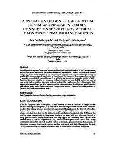
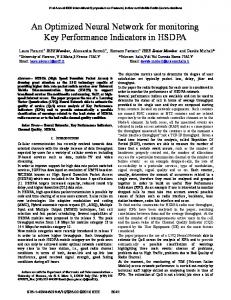
such as RBF and self-organizing feature map (SOFM or SOM), MLP, known as universal approximator, is one of the most popular NNs applied in crash injury severity prediction and data mining in other fields. Consequently, it’s also employed in this study for modeling the underlying non-linear relationship between crash severity and related risk factors. Figure 1 shows the developed MLP structure, in which neurons are fully connected.

x1

1

w1j,i 1

x2

w2k,j

2

1

ψ1

k

ψK

2

x3

3

J

xI 8

I

risk factors

severity levels

hidden layer

9 10 11 12 13 14 15 16 17 18 19 20

Consider a dataset containing N attributes to represent risk factors that may have effects on crash injury severity. In the input layer, each risk factor is represented by a node. A constant node equaling one is included, of which the connection weights with hidden neurons are the biases. Therefore, the number of units, I , in the input layer is I  N 1. Although two or more hidden layers are feasible, a single hidden layer is proposed in the MLP of this study. Villiers and Barnard (1993) found that a single hidden layer is less likely to be trapped at a local minimum during network training. The number of neurons in the hidden layer is assumed to be J . The connection

21

weight between hidden node j,

Figure 1 Structure of the developed MLP

j  1, , J and input node i, i  1, , I is w(1) j ,i .

22

In the output layer, K units  1 , k , K  that respectively express the

23

ordinal severity-outcomes are established. Correspondingly, each observed response

24

yi in the dataset is encoded in a sub-string

25

ok (i )  1 ; else, ok (i )  0 . wk(2),j denotes the weight of the connection between output

26

node k , k  1, , K and hidden node j,

o1 (i ), ok (i ), , oK (i ) . If

j  1, , J .

yi  k , then

Zeng & Huang

1 2 3 4 5 6 7 8

8

3.2 Network training 3.2.1 BP algorithm The BP algorithm modifies the network connection weights according to the calculation error of an example in training dataset each time. A number of shortcuts proposed by Haykin (2009), which may accelerate the convergence of network training process, are adopted in the study. The steps of the proposed BP algorithm are as follows:

9

(2) 1. Initialization. w(1) j ,i ( j  2, , J ; i  1, , I ) and wk , j ( k  1,  , K ; j  1, , J )

10

are randomly selected from two different uniform distributions. The means of both

11

distributions equal zero, and their variances are 1 J and 1 K , respectively.

12 13 14 15

2. Constructing epoch. Randomly arrange the training data in an epoch from one to M . For each pattern (referring to the “observation” in statistical models) m in the epoch, conduct the calculations in step 3 to step 5. 3. Forward calculation. Calculate the outputs of nodes in hidden layer and

16

output layer, H j (m) ,  k (m) , and the calculation errors ek (m) by: I

17

(1)  (1) H j (m)  g j ( (1) j ( m)   w j ,i  xi (m), j ( m)) , i 1

J

18

k(2) (m)   wk(2), j  H j (m),  k (m)  g k (k(2) (m)) , j 1

19

ek (m)  ok (m)  k (m) ,

20

where g j ( ) and gk ( ) are the activation functions of neurons. The hyperbolic

21 22

function, tanh() , which is an odd sigmoid activation function, is used for all neurons in the network.

23

4. Backward calculation. Calculate the local gradients  k(2) (m) and  (1) j ( m) of

24

output layer and hidden layer neurons and the correction values wk(2),j (m) and

25

w(1) j ,i ( m ) of their connection weights by:

26

 k(2) (m)  ek (m) g k (k(2) (m)) ,

27

wk(2), j (m)   (m)wk(2), j (m  1)   (m) k(2) (m) k (m) ,

Zeng & Huang

9

K

1

(2) (2)  (1)  (1) j ( m)  g j ( j ( m))   k ( m) wk , j ( m) , k 1

2

(1) (1) w(1) j ,i ( m )   ( m ) w j ,i ( m  1)   ( m ) j ( m) H j ( m ) ,

3

where  (m) and  (m) are the momentum and step size respectively. Both of them

4

decrease with m :  (m) 

5 6

parameter that controls the decreasing speed. 5. Updating. Update all the connection weights in the network:

7 8 9 10 11 12 13 14 15

16

17 18

19

ns ns  (0) ,  (m)   (0) , in which, ns is a ns  m ns  m

(1) (1) (2) (2) (2) w(1) j ,i  w j ,i  w j ,i ( m) , wk , j  wk , j  wk , j ( m ) ,

6. Checking convergence criteria. At the end of an epoch, if the convergence criterion is met, then the network training is over; else, return to step 2. 3.2.2 CC algorithm The CC algorithm transforms the nonlinear problem for connection weights optimization into a new form, which could be solved by matrix operations directly. The connection weights are decoupled into two matrices, U and V . U consists of all the weights between hidden layer nodes and input layer nodes, (1) (1)  w1,1 , w1,2 ,  (1) (1)  w , w2,2 , U   2,1 ...  ... (1)  wJ ,1 , wJ(1),2 , 

... w1,(1)I   ... w2,(1)I  , ... ...  ... wJ(1), I 

while V consists of all the weights between output layer nodes and hidden layer nodes, (2) (2)  w1,1 , w1,2 ,  (2) (2)  w , w2,2 , V   2,1 ...  ... (2) wK ,1 , wK(2),2 , 

... w1,(2)J   ... w2,(2)J  . ... ...  ... wK(2), J 

20 21 22

The CC updates U and V 1 (the inverse of V ) by the whole dataset each time (Li et al., 2013), which vastly speeds up the calculation process. For a set of training data {(x(l ), d(l )) | l  1, 2,  , L} , the steps of training by CC are as follows:

23

1. Initialization. Randomly generate the J  I matrix U0 and the J  K

24 25

matrix V01 . The number of iteration t  0 . 2. Calculate the values of Yt , Zt , Ut1 , Vt11 successively, according to the

Zeng & Huang

1

10

following equations:

2

Yt   (Ut X) ,

3

Z t  Vt1T ,

4

Vt11  [ Yt  (1   )Z t ]T  ,

5

U t 1X   1[ Yt  (1   )Z t ] .

6 7 8

3. If the convergence criteria are met, the algorithm is done; else, t  t  1 and return to step 2. In the algorithm, X  {x(1), x(2), x( L)} , T  {d(1), d(2), d( L)} , and

9

T  T(TT)1 , where T is the transposition of T . Y and Z are two

10 11 12 13 14 15 16 17 18 19 20 21 22 23 24 25 26

intermediate matrices.  and  are two predetermined parameters, both of which are located in (0,1) .  () is the activation function of hidden neurons and the hyperbolic function is used for its form as in the BP algorithm. For output neurons, the activation function is the identity function. As a consequence, ψ(l )=V (Ux(l )) , l  1, 2, , L .

27

ermax  max  p _ b, q _ b .

28

3.3 Structure optimization To improve the generalization capacity of the NN model and identify the redundant explanatory variables, the N2PFA algorithm is developed to prune the nodes which don’t cause significant deterioration in the network’s accuracy (Setiono and Leow, 2000). The classification accuracies of the training set F and testing set Χ , p and q , are used to evaluate the network’s performance. The N2PFA algorithm has been modified herein to fit its combination with the proposed training algorithm. The following steps describe the detailed pruning process: 1. Train the network with a relatively large number of hidden nodes by CC algorithm. 2. Calculate p and q of the trained NN, and set p _ b  p , q _ b  q ,

3. Retrain the network with J  J  1 , and compute p and q of the

29 30

retrained network. 4. If p  (1   )ermax

31

p _ b  min  p, p _ b , q _ b  min q, q _ b , ermax  max  p _ b, q _ b , and go

32 33

back to step 3; else, keep the previous weights of network connections.  here is a factor to control the chance that a node will be removed.

34

5. For each i (i  1, , I ) , set wi1, j  0( j  1, , J ) and calculate the prediction

and

q  (1   )ermax

,

then

set

Zeng & Huang

1 2 3

11

errors pi and qi . 6. Retrain the network with Xl , which is the matrix X eliminating its l column and pl  mini pi , and compute p and q of the retrained network.

4

7. If p  (1   )ermax and q  (1   )ermax , then remove input node l , set

5

p _ b  min  p, p _ b , q _ b  min q, q _ b , ermax  max  p _ b, q _ b , X  Xl ,

6 7 8 9 10 11 12 13 14 15 16 17 18 19 20 21 22 23 24 25 26 27 28 29 30 31 32 33 34 35 36 37

I  I  1 and go back to step 6; else, keep the previous weights of network connections.

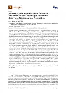
4. DATA PREPARATION The 2006 crash records obtained from the Florida Department of Highway Safety and Motor Vehicles (DHSMV) were used to demonstrate the proposed NN techniques and to compare them with the NNs trained by BP algorithm and an OL model. The analysis focuses on two-vehicle crashes with the whole information on the factors listed in Table 1. A total of 107,464 driver-vehicle units involved in 53,732 crashes were extracted. Among the dataset, only 363 (0.34 percent) involvements resulted in fatalities, and therefore they were combined with incapacitating injuries to constitute the fourth category (incapacitating/fatality) of injury severity, as shown in Table 1. The explanatory factors covered most of the important characteristics of driver, vehicle, roadway and environment. The factors were categorized based on existing definitions in previous studies (Abdelwahab and Abdel-Aty, 2001, 2002; Delen et al., 2006; Huang et al., 2011). With regard to points of impact (POIs), 21 different locations in a vehicle could be recorded in the original Florida crash reports. Apart from undercarriage (no.18), overturn (no.19), windshield (no.20) and trailer (no.21), the others are demonstrated in Figure 2. These locations were divided into four levels depending on their estimated effects on injury severity. The first level comprises nine POIs (nos. 1-2, 5-7, 9-10, 14, 21), most of which are farthest from the driver’s seat, such as the front and rear passenger side of the vehicle. Five POIs (nos. 3, 8, 11, 15, 17) which are closer to the driver’s seat than POIs in Level 1 are grouped as Level 2. Level 3 POIs (nos. 4, 12-13, 18, 20) are even closer to the driver’s seat, including the windshield, front passenger side, and front driver side of the vehicle. Two POIs (nos. 16, 19) with the highest risk of driver injury are grouped as Level 4. Huang et al. (2011) devised the detailed categorization process.

Zeng & Huang

1

12

Table 1 Descriptions of variables for modeling Variables

Description

Descriptive statistics

Response variables Injury severity

No injury/property damage only=1

No injury: 54.76%

Possible injury=2

Possible injury: 24.84%

Non-incapacitating injury=3

Non-incapacitating injury: 14.77%

Incapacitating injury/ fatality =4

Incapacitating injury/ fatality: 5.64%

Explanatory variables Driver age

65: 9.40%

Male=1

Male: 56.36%

Female=2 (reference case)

Female: 43.64%

Alcohol/drug

No drink or drugs=1

No drink or drugs: 96.05%

use

Drink or drugs=2 (reference case)

Drink or drugs: 3.95%

Safety

No use of safety equipment=1

No use of safety equipment: 5.15%

Equipment

Use of safety equipment=2 (reference case)

Use of safety equipment: 94.85%

Driver fault

At fault=1

At fault: 41.59%

Not at fault=2 (reference case)

Not at fault: 58.41%

1996-2006=1

1996-2006: 76.03%