period (Buongiorno and Gilless 1987). For brevity, this formulation will be referred to as the âforestry-DP.â The forestry-DP formulation requires specification of a ...
A STAND OPTIMIZATION MODEL DEVELOPED FROM DYNAMICAL MODELS FOR DETERMINING THINNING STRATEGIES Oliver Chikumbo, Iven M.Y. Mareels, and Brian J. Turner1
ABSTRACT. —The “curse of dimensionality” common in dynamic programming (DP) formulations of the thinning strategy problem has previously been overcome by applying the neighborhood storage location concept. However, several forest analysts are aware that the solutions obtained in this manner are suboptimal. Even worse, there is no easy way of determining how far a particular solution may be removed from optimality. Here we present an approach using dynamical models. The application of control theory can then be used to effectively overcome the dimensionality problem. Moreover, we may exploit optimization routines capable of guaranteeing optimality. In this paper, we describe how this approach has been used to address the thinning problem for Pinus radiata D. Don plantations in the Australian Capital Territory.
INTRODUCTION The management of a plantation forest includes, among other things, defining operational area units and estimating the growth and yield for each unit under a set of alternative activities (harvesting/silvicultural strategies). Each land unit may have different levels of site productivity, making it difficult to determine an optimal harvesting strategy at a stand level. Forest analysts have used multistage optimization to determine the harvesting strategies that best satisfy specific objectives. Because of the daunting mathematical extent of optimization formulations, “simulators” have been used to determine silvicultural strategies, but these cannot indicate whether the outcomes are optimal or suboptimal. Simulators are computer-based, decision-support systems that enable experimentation on a model rather than on the forest itself to evaluate the forest behavior under different conditions (Ljung 1987). Multistage optimizers enable control or guidance, generally defined as the directed influence, on a dynamic system to achieve a desired outcome (Luenberger 1969). Dynamic programming (DP) is a technique commonly used by forest analysts to solve multistage optimization problems for harvesting stands. However, the technique has not been implemented without presenting its own difficulties that Bellman (1957) called the “curse of dimensionality.” The curse of dimensionality results from the need to define all the possible states at each stage of a DP formulation that can be computer-memory demanding, even for small DP problems. To counter the dimensionality problem, forest analysts have developed a DP formulation that requires the user to specify possible states that are common to all the finite stages in the planning period (Buongiorno and Gilless 1987). For brevity, this formulation will be referred to as the “forestry-DP.” The forestry-DP formulation requires specification of a finite number of states (usually two to three states at each stage). The choice of these states is based on expert knowledge of the forests in question. The stages are normally specified at equal intervals of 5 to 10 years. This neighborhood storage technique is very limiting in that decisions are confined to long interval points and there is no exhaustive search of the states at each stage. Therefore, there is no guarantee of finding a global optimum over the planning period and there is no easy way of checking whether the solution is suboptimal or optimal. The forestry-DP formulation can be described as a heuristic method combined with recursive optimization. In contrast, DP employs the embedding technique that enables an exhaustive search of all the possible states at each stage in a backward recurrence mode.
1
Oliver Chikumbo, growth and yield modeler and research fellow, Bureau of Resource Sciences, P.O. Box E11, Kingston, ACT 2600, Australia. Iven M.Y. Mareels, Professor and Head of Department, Department of Electrical and Electronic Engineering, University of Melbourne, Parkville, Victoria 3052, Australia. Brian J. Turner, Reader, Department of Forestry, The Australian National University, Canberra, ACT 0200, Australia.
1
Arthaud and Klemperer (1988) concluded that neighborhood storage combined with a forward recursion optimization resulted in violation of the principle of optimality; this formulation led to loss of paths that would have been optimal over the long run, but were discarded because of lower values (generated through thinning). Some authors (e.g., Anderson and Bare 1994; Arthaud and Klemperer 1988; Arthaud and Warnell 1994; Pelkki 1994; Valsta 1994) have deduced that they may be just achieving local optima. Chen et al. (1980) concluded that some of the problems of the forestry-DP formulation were caused by the use of inappropriate growth models that did not relate directly to the decision variable and the lack of a clear definition of the conditions that had to be met for optimality. In this paper, basal area models are developed for Pinus radiata D. Don plantations in the Australian Capital Territory (ACT) from time-series data describing basal area and stand density. These models are discrete-time “dynamical models.” Dynamical models are common in the field of systems engineering and describe dynamic systems where control and controlled variables are identified. For a first-order, discrete-time dynamical model, the current observation at time t depends on the previous observation at time t-1. For a second-order model, the observation at time t is dependent on the previous observations at times t-1 and t-2. Time is implicit in a discretetime dynamical model and is used as an integer to indicate equidistant observations (Chikumbo 1997). Dynamical models may be represented using input/output (thinning/basal area) variables only or using input/state/output (thinning/basal area, stand density/basal area) variables. The input/state/output representation enables one to steer a dynamic system from an initial state to a final state via the control action. A multistage optimization problem for determining optimal thinning strategies was formulated based on a state space model and solved using the maximum principle (MP), a technique similar to DP (Pontryagin 1956).
Data The softwood plantation resource in the ACT (149° E, 35°19 min) has a net productive area of 14,500 hectares (ha) with P. radiata as the main species. The plantations were established on degraded pastures and land cleared of eucalypt forest. The annual rainfall in the ACT ranges from 610 to 1,140 millimeters (mm). The soils are generally poor and are derived from acid volcanics, granodiorites, and sediments. The plantation area comprises Kowen, Pierce’s Creek, Stromlo, and Uriarra forests. A summary of rainfall and geology of the four forest areas is given in Table 1. Table 1.—Rainfall and geological characteristics of the forests in the Australian Capital Territory Forest Area
Rainfall
Geological Characteristics Age
Description
± 650 ± 700 ± 800
Ordovician Upper Silurian Silurian to Devonian
mostly slates variable, mainly acid volcanics and porphyry mostly granite to granodiorite
± 800 ± 850
Upper/Middle Silurian Ordovician
Uriarra volcanics/Paddy River volcanics sedimentary slates
mm Kowen Stromlo Pierce’s Creek Uriarra East Uriarra West
A 5-year soil survey program is currently being undertaken by ACT Forests Branch on a 150 by 150-meter (m) grid. This will provide useful information for site-specific silvicultural management. The data used for model development were collected from a number of permanent yield plots established in the 1940’s through the 70’s by the then ACT Forests Branch, Australian Forestry School, and Commonwealth Forest
2
Research Institute. The plots ranged in size from 0.01 to 0.1 ha and usually had a rectangular shape. The stocking densities at establishment ranged from 750 to 2,990 stems ha-1. Thinnings were mainly frequent and light, making it difficult to estimate their effects on growth volume production. In total, the data were from 240 plots that had been measured on 3,637 occasions. Table 2 summarizes the data from the four forest areas in the ACT. Table 2.—Minimum, mean, and maximum values of stand variables of the four ACT forest areas Forest Area
Number of Plots
Age
min
mean
Site Index
max
- - - - years - - - Kowen Pierce’s Creek Stromlo Uriarra
72 50 3 115
4 5 9 4
22.8 22.8 23.1 20.9
44 57 39 51
min
mean
Basal Area
max
min
20.9 22.5 20.2 24.9
25.6 27.2 22.2 31.7
max
- - - m2 ha-1 - - -
-----m----16.1 18.7 19.1 16.5
mean
Stand Density
1.7 1.1 9.4 0.5
31.4 30.9 27.6 31.5
79.9 58.6 38.4 99.9
min
mean
max
- - - stems ha-1 - - 151 51 173 9
713 679 588 774
2,903 5,182 971 2,976
MODEL DEVELOPMENT There was no consistency in timing and intensity of thinning from the permanent growth plots. Therefore, to develop a basal area model responsive to thinning at different intensities and timing, we selected prolonged periods of basal area measurements between any two successive thinnings from the permanent plots. Interpolation was carried out for any two successive data points that were more than 1 year apart so as to have annual records. We did this for each of the forest areas. Basal area models were identified, using subsets of the series of basal area measurements from various plots for each of the forest areas. Kowen, Pierce’s Creek, Stromlo, and Uriarra had 10, 19, 5, and 21 basal area models, respectively. These models with their statistical properties are given in appendix I. The identification process of the basal area model consisted of a two-step approach: 1.
For each subset of the series of basal area measurements, we identified a first order, discrete-time dynamical model that explained the general basal area growth trend.
2.
We regressed the parameters of the models in 1 against initial stand density and site index for each forest area. The subsets of basal area measurements combined for each forest area had a small range of site indices, which resulted in site index not being used in the analysis. Therefore, we modeled these parameters using polynomials that were functions of stand density for each forest area.
The model was as follows: (1)
BA(t) = aBA(t-1) + b
where t = time (years); x = initial stand density (stems ha-1); BA = stand basal area (m2ha-1); (2)
a = f(x);
(3)
b = f(x).
Table 3 gives the polynomials for parameters a and b for the four forest areas.
3
Table 3.—Forest areas, their polynomial functions for a and b, and R-squared values Forest Area Kowen Pierce’s Creek Stromlo Uriarra
Polynomial Functions
R-Squared Values
a=-0.0000000486x2+0.0000813x+0.868 b=0.00000132x2-0.00207x+5.085 a=-0.0002x+1.0339 b=0.0102x-0.5463 a=-0.0000000956x2+0.0002x+0.814 b=0.0000123x2-0.01718x+9.908 a=-0.000037x+0.9941 b=0.002x+1.7606
0.80 0.78 0.82 0.92 0.68 0.81 0.77 0.89
A simulation of the basal area models for three initial stand densities of 500, 1,000, and 1,500 stems ha-1 showed that a high initial stocking achieved a basal area asymptotic limit (as dictated by site quality) sooner than a lower initial stocking (see Fig. 1). Stromlo forest showed similar trends but could not be simulated using the same initial stocking as the rest of the other forests. This was because the Stromlo model was based on only five models with 971 stems ha-1 as the highest stocking density. Therefore, the Stromlo model could not be reliably extrapolated beyond 1,000 stems ha-1. A low stocking showed a slower rate in taking advantage of the available site compared with the high stocking. For all the forest areas, the basal area gain was not substantial for a higher stocking. The comparison between high stocking and low stocking for the ACT forests suggests that thinning has to be minimal otherwise the residual trees may not have the ability to fully occupy the site (maximizing basal area per tree). Rotations also have to be as long as possible for value production regimes such that the final crop can reach the largest size that a site can allow.
4
KOWEN FOREST
PIERCES CREEK FOREST
50
70 60 per ha)
50 40
2
30
2
per ha)
40
30
20 =500 =1,000 =1,500
10 0 0
10 20 age (years)
10 0
30
0
70
50
60 per ha)
60
40 30
50 40
10 20 age (years)
30
URIARRA FOREST =500 =1,000 =1,500
2
per ha)
STROMLO FOREST
2
=500 =1,000 =1,500
20
30 20
=500 =700 =1,000
10 0 0
10 20 age (years)
20 10 0
30
0
10 20 age (years)
30
Figure 1.—Simulation of basal models for three initial stand densities on each of the ACT forest areas. Kowen forest showed very little variation in basal area growth from the three simulations. The area has poor, shallow soils and low rainfall. The ACT Forests Branch has confirmed that they aim to maintain basal area at 20 m2 ha-1 because of low productivity in this forest area. Pierce’s Creek and Uriarra forests showed comparatively higher basal areas at age 30 because of the relatively better soils and rainfall.
Optimal Control We considered the following optimal thinning problems,:
u( t ) * BA( t ) t = 0 x( t ) n
(4) minimize Jvol( u , z ) = − ∑ u ,z
for volume production and,
5
u( t ) BA( t ) * * BA( t ) x( t ) t = 0 x( t ) n
(5) minimize Jval( u , z ) = − ∑ u ,z
for value production. The cost functional Jvol is a measure of the total basal area harvested. The initial stocking is expressed as z, which has to be optimized. These minimizations are subject to the following constraints, the system equations (dynamics), (6)
x(t+1) = x(t) - u(t)
(7)
BA(t+1) = a(x(t))BA(t) + b(x(t))
where a(x) and b(x) are defined in Table 2. The above system equations have to be completed with the initial conditions, (8)
x(0) = z > 0, BA(0) = 0,
terminal constraint, (9)
x(n) = u(n),
and upper and lower bounds on thinning: (10)
0 ≤ u( t ) ≤ x( t ), ∀t = 0 ,..., n -1
For the above formulation n=25, but this also could have been left as a free variable to be optimized. Notice that u(t)/x(t) indicates the fraction of trees harvested at time t. The cost functional Jval puts more emphasis on bigger trees, due to the presence of the weighting factor BA(t)/x(t) which is the average basal area per tree. Given more information on costs of establishment, thinning, pruning and so on, an economic component can be incorporated in the cost functional to be optimized as well as in the constraints that have to be satisfied. A software package called MISER (Jennings et al. 1990) was used to solve the thinning optimization problem. The algorithm in MISER uses the maximum principle technique for solving optimal control problems. The maximum principle employs the Kuhn-Tucker method (Dixon 1972) for minimizing a function subject to equality and inequality constraints. This optimization problem can be viewed as the minimization of a functional Jvol or Jval of n+2 variables, i.e., and u(0),…, u(n) and z, subject to a set of equality and inequality constraints as described in equations 6 through 10. For all of these constraints, the appropriate Lagrangian multipliers can be determined and then optimized as an augmented cost functional. This can be solved efficiently using a gradient-based search algorithm, such as in MISER. It is important that the functions used in formulating the optimization problem be sufficiently smooth with respect to the control variables to allow for the differentiation. This is the case with the thinning problem where all functions are at least twice differentiable with respect to the control variable. By formulating the problem in this manner, one can solve the necessary local optimality conditions for a candidate optimal thinning strategy that can be refined to satisfy all constraints. This can be achieved without the need for a global search, thus alleviating the dimensionality curse. A solution found this way (by MISER) will be a local minimum of the optimization problem at hand. Sometimes there is no guarantee that the locally optimum solution is the global minimum. This is not an issue with problem formulation 6 through 10 because there is no other minimum for such a relatively simple formulation (only two state variables).
RESULTS Kowen and Stromlo forests had similar MISER outputs. Both value and volume production regimes had an initial stocking of 677 stems ha-1 with a final crop of 122 and 140 stems ha-1 respectively. Thinning was light and annual.
6
We optimized the value production formulation again with a terminal constraint set at ages 30 and 35. In both cases, the crop was maintained at 122 stems ha-1. This suggested that the final crop has to be retained for as long as possible for the residual trees to take complete advantage of the available site. The interpretation of the MISER output was that an initial stocking of 600 to 700 stems ha-1 be adopted and light thinnings carried out at stages best determined by including financial costs in the optimization formulation. The final crop may be harvested at any time from age 25 for volume production and retained for longer periods for value production (i.e., rotation lengths of 35 years or more). ACT Forests Branch is moving towards lower stocking regimes and establishments of 650 stems ha-1 in Kowen forest. Pierce’s Creek and Uriarra forest areas had similar thinning regimes. There were minimal benefits in thinning for both value and volume production regimes such that exercise became one of optimizing for the initial number of trees as for Kowen and Stromlo forests. The output from MISER for a volume production regime was one with an initial stocking of 880 stems ha-1 and an annual thinning of 37 stems ha-1 until there was no crop at age 25. This result was interpreted as an initial stocking of the order of 800 to 900 stems ha-1 with light thinnings again best determined by financial formulation of the thinning problem. For the value production regime, the MISER output had an initial stocking of 677 stems ha-1 with an annual thinning of 22 stems ha-1 and a final crop of 122 stems ha1 at age 25 that should be maintained as long as possible. The interpretation was that value production had an initial stocking of 600-700 stems ha-1 with light thinnings, as suggested for Kowen and Stromlo. ACT Forests Branch agreed with these conclusions because the Pierce’s Creek and Uriarra forest areas have comparatively better soils and rainfall than Kowen and Stromlo forests. In fact, fertilization is an option for ACT Forests Branch. At this stage there is no pulpwood market, and therefore it is important to estimate the initial planting density. The thinning strategy model has a huge potential as a management tool in addressing silvicultural questions that would normally require experimental plots to be established and analyzed over a number of years. Financial parameters incorporated in the model would make the assessment more realistic.
CONCLUSIONS The thinning problem has been solved using dynamical models and formulating a multistage optimization problem. The curse of dimensionality problem has not been encountered as a result of using the maximum principle, despite treating each year as a decision stage. The interpretations of the MISER output suggested similarities with the current recommendations of silvicultural strategies to be adopted by the ACT Forests Branch, which have been derived from years of experience by field foresters.
ACKNOWLEDGMENTS We thank ACT Forests Branch for providing us with data and other relevant information. We are also grateful to Dr. Ride James (ANU, Department of Forestry) for helpful comments. We are greatly indebted to the Bureau of Resource Sciences for their major contributions in providing the funding and environment for carrying out this research.
LITERATURE CITED ANDERSON D.J., AND B.B. BARE. 1994. A dynamic programming algorithm for optimization of uneven-aged forest stands. Canadian Journal of Forest Resources 24: 1758–65. ARTHAUD, G.J., AND W.D. KLEMPERER. 1988. Optimising high and low thinnings in loblolly pine with dynamic programming. Canadian Journal of Forest Resources 18: 1118–22.
7
ARTHAUD, G.J., AND D.B. WARNELL. 1994. A comparison of forward-recursion dynamic programming and A* in forest stand optimization. In Management systems for a global economy with global resource concerns, eds. Sessions, J., and Brodie, J.D. Pacific Grove, CA. BELLMAN, R.E. 1957. Dynamic programming. Princeton, NJ: Princeton University Press. BUONGIORNO, J., AND J.K. GILLESS. 1987. Forest management and economics. New York: Macmillan Publishing Company. CHEN, C.M., D.W. ROSE, AND R.A. LEARY. 1980. How to formulate and solve optimal stand density over time problem for even-aged stands using dynamic programming. Gen. Tech. Rep. NC-56. U.S. Department of Agriculture, Forest Service. CHIKUMBO, O. 1997. Applicability of dynamical models and theoretical control methods in tree growth prediction and planning. Ph.D. thesis. Australian National University. DIXON, L.C.W. 1972. Nonlinear optimization. The English Universities Press Ltd. JENNINGS, L.S., M.E FISHER, K.L. TEO, AND C.J. GOH. 1990. MISER: Optimal control software—Theory and user manual. W.A. 6020, Australia: EMCOSS Pty. Ltd. LJUNG, L. 1987. System identification: Theory for the user. Englewood Cliffs, NJ: Prentice-Hall, Inc. LUENBERGER, D.G. 1979. Introduction to dynamic systems: Theory, models, and applications. New York: Wiley. MATHWORKS, INC. 1992. MatLab: High performance numeric computations and visualisation software, reference guide. Natik, MA: Cochituate Place. PELKKI, M.H. 1994. Exploring the effects of aggregation in dynamic programming. In Management systems for a global economy with global resource concerns, eds. Sessions, J., and Brodie, J.D. Pacific Grove, CA. PONTRYAGIN, L.S. 1959. Optimal regulation processes. Uspekhi Matem. Nauk 14:1, (in Russian). English translation in Am. Math. Soc. Trans, Ser.2, Vol. 18: 321–39, 1961. VALSTA, L.T. 1994. Silvicultural guidelines based on optimization with stochastic price and growth. In Management systems for a global economy with global resource concerns, eds. Sessions, J., and Brodie, J.D. Pacific Grove, CA.
8