continuous state-space to represent incremental progress and intermediate .... utterances âI'll willingly marry Marilynâ and âour lawyer will allow your rule,â each ...
GAUSSIAN PROCESS DYNAMICAL MODELS FOR NONPARAMETRIC SPEECH REPRESENTATION AND SYNTHESIS Gustav Eje Henter1,∗
Marcus R. Frean2
W. Bastiaan Kleijn1,2
1
2
School of Electrical Engineering, KTH – Royal Institute of Technology, Stockholm, Sweden School of Engineering and Computer Science, Victoria University of Wellington, New Zealand ABSTRACT
We propose Gaussian process dynamical models (GPDMs) as a new, nonparametric paradigm in acoustic models of speech. These use multidimensional, continuous state-spaces to overcome familiar issues with discrete-state, HMM-based speech models. The added dimensions allow the state to represent and describe more than just temporal structure as systematic differences in mean, rather than as mere correlations in a residual (which dynamic features or AR-HMMs do). Being based on Gaussian processes, the models avoid restrictive parametric or linearity assumptions on signal structure. We outline GPDM theory, and describe model setup and initialization schemes relevant to speech applications. Experiments demonstrate subjectively better quality of synthesized speech than from comparable HMMs. In addition, there is evidence for unsupervised discovery of salient speech structure. Index Terms— acoustic models, stochastic models, nonparametric speech synthesis, sampling 1. INTRODUCTION Hidden Markov models (HMMs) [1] constitute the dominant paradigm in model-based speech recognition and synthesis (e.g., HTS [2]). HMMs are probabilistic, allowing them to deal with uncertainty in a principled manner, and strike an attractive balance between complexity and descriptive power: they avoid restrictive assumptions such as limited memory or linearity, but can still be trained efficiently on large databases. Unfortunately, HMMs are not satisfactory stochastic representations of speech feature sequences [3]. Sampling from HMMs trained on speech acoustic data reveals several shortcomings of the model, in that durations are incorrect and the sound is warbly and unnatural. Contemporary model-based speech synthesis systems, HMM-based or not, therefore do not sample from stochastic models for signal generation. In this paper we introduce a new paradigm of nonparametric, nonlinear probabilistic modelling of speech, as exemplified by Gaussian process dynamical models (GPDMs). ∗ This research is supported by the LISTA project. The project LISTA acknowledges the financial support of the Future and Emerging Technologies (FET) programme within the Seventh Framework Programme for Research of the European Commission, under FET-Open grant number: 256230.
This approach has the potential to overcome all principal issues with HMMs and provide more realistic acoustic models. Like HMMs, GPDMs may later serve as building blocks for constructing arbitrary speech utterances. In the remainder of the text, we motivate and describe GPDMs in the context of acoustic models of speech signals, and present concrete results from a synthesis application. 2. INTRODUCING GPDMS FOR SPEECH We here explain the benefits of moving from Markov chains to continuous, multidimensional state-spaces, and introduce GPDMs as nonparametric dynamical models of speech. 2.1. Continuous, multidimensional state-spaces Let Y =(Y 1 . . . Y N ) be a sequence of observations, here speech features, and let X=(X 1 . . . X N ) be the corresponding sequence of unobserved latent-state values. The features are typically continuous and real, y t ∈RD , with D between 10 and 100. We consider Y a D×N matrix random variable. HMMs have a discrete state-space, xt ∈ {1, . . . , M } ∀t. This is sufficient to model piecewise i.i.d. processes, but is not a good fit for speech since 1) HMMs have stepwise constant evolution, while speech mostly changes continuously, and 2) the implicit geometric state-duration distribution of the underlying Markov chain has much greater variance than natural speech sound durations. Dynamic features and hidden semi-Markov models [4] have been proposed to deal with issues 1) and 2) separately, respectively. Both shortcomings can however be addressed simultaneously, by considering a continuous state-space to represent incremental progress and intermediate sounds [5]. This is the approach explored here. Typical speech HMMs use left-right Markov chains to encode long-range dependencies between features at different times, specifically the sequential order of sounds in an utterance. Other dependence-modelling is less structured. Shortrange time-dependencies can be described as time-correlated deviations from the state-conditional feature mean, e.g., using dynamic features [3]. This enables gradual changes in expected value. Variation between comparable times in distinct realizations is usually only modelled as Gaussian deviations from a single state-conditional mean value.
In practice, these correlation-based approaches fail to capture important structure in speech variation, and do not produce realistic speech samples [6]. The sampled speech has a rapidly-varying, warbly quality to it due to the large magnitude of the noise-driven deviations from the feature mean. To obtain more pleasant-sounding output, speech synthesizers therefore generally avoid sampling, and only produce the most likely output sequence. This is known as maximum likelihood parameter generation (MLPG) [7]. The models considered here can use multidimensional state-spaces xt ∈RQ to represent structured differences between realizations. The added state-space dimensions may for instance track different pronunciations for the same utterance, e.g., stress-dependent pitch and formant evolution. As both the continuous state-space and the extra dimensions give us flexibility to explain more empirically observed variation as systematic differences in mean, less variability will be attributed to residual, random variation. The estimated noise magnitude will thus decrease, making samples less warbly and more realistic. We now consider a specific model on such state spaces, based on Gaussian processes. 2.2. Gaussian process dynamical models A dynamical model for Y is defined by 1) an initial state distribution fX 1 (x1 ), 2) a stochastic mapping fX t+1 |X t (xt+1 | xt ) describing state-space dynamics, and 3) a state-conditional observation distribution fY t |X t (y t | xt ). In speech, xt may represent the state of the speaker—particularly the sound being produced—while y t is the current acoustic features. In a simple HMM describing a speech utterance or phone (for synthesis), fX t+1 |X t is usually a left-right Markov chain. The output fY t |X t is often Gaussian for synthesis tasks, but GMMs are common in recognition. In this paper, however, both fX t+1 |X t and fY t |X t will be modelled as continuousspace densities, using stochastic regression based on Gaussian processes (GPs). (For a review of Gaussian processes please consult [8].) The resulting construction is known as a Gaussian process dynamical model, GPDM [9, 10]. For the output mapping fY t |X t , GPDMs use a technique known as Gaussian process latent-variable models (GP-LVMs) [11]. These assume the output is a product of Gaussian processes, one for each y t -dimension, with a shared covariance kernel kY (x, x0 ) that depends on latent variables X t . The processes are conditionally independent given xt , similar to assuming diagonal covariance matrices in conventional HMMs. The conditional output distribution becomes f (y|x, β, w)= √
1 (2π)DN |K Y (x, β)|D
·
QD
d=1
2 T wd exp(− 21 wd yd K −1 Y (x, β)yd ),
(1)
where the kernel matrix has entries (K Y )t, t0 = kY (xt , xt0 | β), β being a set of kernel hyperparameters. The scale factors wd compensate for different variances in different output dimensions. The entries of X are assumed Gaussian and i.i.d.
Using GP-LVMs for the output mapping essentially assumes that acoustic features y t have similar characteristics (mean and standard deviations) for similar speech states xt , e.g., the same phone being spoken, though the details depend on the chosen kY . This is similar in principle to HMMs, but is more flexible and does not assume that xt is quantized. GP-LVMs were designed as probabilistic, local, nonlinear extensions of principal component analysis (PCA), and MAP estimation in a GP-LVM will therefore attempt to attribute as much as possible of the observed acoustic y-variation as due to variations in the underlying speaker state X t . GP-LVMs assume X is i.i.d., and have no memory to account for context or to smooth estimated latent-space positions over time. GPDMs endow the GP-LVM states with simple, first-order autoregressive dynamics f∆X t |X t , so that ∆X t =X t+1 −X t is a stochastic function of X t . (Higherorder dynamics and other constructions are also possible [9].) Specifically, the next-step distributions for the ∆X t components are assumed to be given by separate Gaussian processes (with a shared kernel kX (x, x0 )), conditionally independent of other dimensions and of Y given xt . The joint probability distribution is more involved than for the GP-LVM, as the dynamics map a space onto itself. It can be written f (x|α)=fX 1 (x1 ) √
1 (2π)Q(N −1) |K X (x, α)|Q T · exp(− 12 tr(∆xK −1 X (x, α)∆x ))
(2)
where ∆x=(x2 − x1 , . . . , xN − xN −1 ). This distribution is not Gaussian as K X depends on x, and fair sampling requires Metropolis-type algorithms. An approximation called mean prediction [9] exists for sequentially generating latent-space trajectories of high likelihood, analogous to MLPG. Using GPs to describe state dynamics represents an assumption that the state of the speaker, and thus the acoustic output, evolves similarly when the state is similar, quite like how HMMs work but without the discretization. By endowing all hyperparameters with priors, a fully Bayesian nonparametric dynamical model is obtained. MAP estimating the unobserved GPDM variables α, β, W , and X is straightforward using gradient methods. However, there are many local optima and the estimated latentspace trajectories are typically quite noisy, since the GPDM tries to place as much variation as possible in the latent space. To prevent such overfitting, the unknown X can be integrated out using Monte-Carlo EM, leading to low process noise and highly realistic samples in a motion capture application [10] (video). Alternatively, one may choose a fixed α with low noise to obtain smooth dynamics, as we do here. 3. IMPLEMENTING GPDMS FOR SPEECH GPDMs were first introduced to model motion capture data, and we are unaware of any prior applications to speech.1 We 1 A reviewer noted that [12] provides an application to ASR; it was published while this paper was in review.
here discuss specific issues in using GPDMs as speech acoustic models, and propose an initialization scheme for sequential signals such as speech utterances. 3.1. Feature representation To create speech features suitable for GPDMs and to synthesize speech, we employed the widely used STRAIGHT system [13]. The STRAIGHT analysis yields: 1) an F 0 contour with voiced/unvoiced indication, 2) a filter spectrum, and 3) an aperiodicity spectrum. To get a more compact feature set, we represented the two spectra by 40 and 10 MFCCs, respectively, and downsampled the features to 100 fps. We also removed the mean of each component over the dataset. The relative scale of the STRAIGHT outputs is arbitrary. Even though the scaling factors w in (1) can in principle compensate for different feature SNRs, we normalized all dimensions to have unit noise magnitude, as this is beneficial for PCA-based initialization schemes. Component SNRs were estimated by fitting a third-order AR-process to each dimension and looking at the standard deviation of the driving noise. The HTS system [2] uses a mixture of continuous and discrete distributions to represent voiced pitch or unvoiced excitations. This is unsuitable for GPs, which are designed for continuous data spaces. For simplicity, we have restricted ourselves to voiced speech in this initial work. 3.2. Covariance functions Because the feature data mean has been removed it is appropriate to use zero-mean GPs. We then only need to specify kX and kY to have a fully defined model. For the dynamics, we chose a simple squared exponential (RBF) kernel with a noise term, � � α 2 2 kX (x, x0 ) = α1 exp − kx − x0 k + α3−1 δx, x0 . (3) 2 Linear and higher-order kernel terms are left as future work. A similar RBF kernel with a noise term is an appealing choice also for kY , to model smooth output with some residual variation. Rapid changes and localized discontinuities such as plosives can be modelled with, e.g., neural network kernel functions [8], though that has not been pursued here. 3.3. Advanced initialization As the likelihood function for the latent x has many local optima, the starting position x(0) in MAP is highly influential in determining the quality of the final model. We hence went to some lengths to compute a starting position that well expresses our expectations on process behaviour. Initializing the latent-space variable trajectory by PCA, as in [10], ignores the time dimension of the data and produces a model where acoustically similar frames will evolve similarly regardless of utterance position, like in a (non-hidden) Markov chain. This is precisely what we strive to avoid.
As the most important variation in speech occurs along the time dimension, we initialized the first latent coordinate by the time from utterance start, as an indicator of progress through the sentence. Multiple training utterances were aligned by dynamic time warping. Remaining x-dimensions were initialized by PCA, so that points at comparable times were spaced closer or farther according to acoustic similarity. As the scale of the first latent dimension is arbitrary rel ative to other axes, it was rescaled according to ∆x1 (0) 2
1 ∆x2:Q (0) 2 , to have comparable RMS ∆x-magni= Q−1 tude to the remaining dimensions. Finally, the mean
was
removed and all axes were rescaled equally so that x(0) 2 =DN , to match the Gaussian prior mean and variance. 4. EXPERIMENTS In order to assess the properties of GPDMs as stochastic models of speech, we performed experiments with utterance synthesis and speech representation, and contrasted the results against comparable HMMs. 4.1. Speech generation For synthesis applications, we are interested in the quality of samples and maximum probability output of our speech models. This was investigated in a subjective listening test. The test was based on a dataset containing the fully voiced utterances “I’ll willingly marry Marilyn” and “our lawyer will allow your rule,” each spoken three times by a single, male speaker. Separate models were trained on the voiced frames of each of the two utterances. For GPDMs, we set Q=1, fixed the dynamics hyperparameters at 20 dB SNR to get smooth latent trajectories, and performed 1000 gradient updates for training. Left-right HMMs with 40 states per second were also trained on the data using the Baum-Welch algorithm. By not including dynamic features we obtain comparable models that cannot pass any information between frames, apart from the current position within the utterance. The listening test included the voiced sections of raw database utterances, speech resynthesized from training-data features, mean-predicted output and random samples2 from the GPDM, and MLPG and random samples from the HMMs. Eight subjects were asked to rate these deterministic and stochastic signal sources on a scale from 0 (completely unnatural) to 100 (completely natural) using a MUSHRA-like interface. The resulting scores are summarized in table 1. In the test, subjects judged GPDM output as more natural than that of HMMs, both for deterministic signals and sampled output. The differences are significant according to paired t-tests (p=0.0017 and 0.014, respectively). GPDM duration modelling, in particular, is noticeably better as the continuous state-space can represent incremental progress 2 We used a fast, approximate procedure for sequentially generating latent trajectories. It is similar to mean prediction, but each new point is sampled from the Gaussian next-step distribution, rather than just taking its mean.
Sound source Database speech Resynthesized GPDM mean pred. GPDM sampled HMM MLPG HMM sampled
“I’ll willingly...” Mean St. dev. 100 0 66 19 74 15 25 11 63 13 16 18
“Our lawyer...” Mean St. dev. 100 0 70 16 78 18 23 16 62 15 10 10
discrete-state hidden Markov models of speech. Such representations can be constructed without restrictive parametric assumptions using Gaussian process dynamical models. The advantages of nonparametric speech modelling through GPDMs include automatic structure discovery and more natural synthesized speech, as affirmed by experimental evidence. Further efforts are needed, particularly for the training stage, to realize the full potential of the models and to apply them as building blocks in arbitrary speech synthesis. Work is presently underway to address these limitations. We are also investigating adding dynamic features for improved, framecorrelated noise modelling.
Table 1. Naturalness scores from listening test.
1.5 1
6. REFERENCES
x3t
0.5 −1.5 0 −1 −0.5
−0.5 0
−1
0.5 −1.5 −3
1 −2
−1
0
1
2
1.5
x2t
3
x1t
Fig. 1. Latent-space trajectories separated in 3D. through the utterance. Sampling consistently scored below deterministic output due to the unnatural, uncorrelated noise. Interestingly, subjects preferred GPDM mean-predicted output over speech resynthesized from the training data features (p=0.038). A possible explanation is that the meanpredicted output is smoother and more stylized. 4.2. Speech representation In a second experiment, we explored how the additional statespace dimensions in GPDMs can represent multimodal distributions and speech variability. For this, we used six examples of the utterance “our lawyer will allow your rule,” three times pronounced with the stress on “lawyer,” and three times instead stressing the word “allow.” If not handled properly, data inconsistencies like this can degrade the quality of traditional speech synthesis systems. However, a GPDM with Q=3 trained on the data correctly separates the two prosodic variations in the latent space— shown in blue (on top) and red (below) in figure 1—and can represent both pronunciation patterns simultaneously. At the same time, the three curves from each variant are placed close together, meaning that information is shared between these examples and a common stochastic representation has been learned. Note that this structure was not imposed beforehand (as is typically necessary to model the situation with an HMM), but was recovered automatically from the data. 5. CONCLUSIONS AND FUTURE WORK We have described how models with continuous, multidimensional state-spaces can avoid the shortcomings of traditional,
[1] L. R. Rabiner, “A tutorial on hidden Markov models and selected applications in speech recognition,” Proc IEEE, vol. 77, no. 2, pp. 257–286, 1989. [2] H. Zen, T. Nose, J. Yamagishi, S. Sako, T. Masuko, A. W. Black, and K. Tokuda, “The HMM-based speech synthesis system version 2.0,” in Proc ISCA SSW6, 2007, vol. 6, pp. 294–299. [3] H. Zen, K. Tokuda, and T. Kitamura, “Reformulating the HMM as a trajectory model by imposing explicit relationships between static and dynamic feature vector sequences,” Comput Speech Lang, vol. 21, no. 1, pp. 153–173, 2007. [4] H. Zen, K. Tokuda, T. Masuko, T. Kobayashi, and T. Kitamura, “Hidden semi-Markov model based speech synthesis,” in Proc ICSLP 2004, 2004, pp. 1393–1396. [5] G. E. Henter and W. B. Kleijn, “Intermediate-state HMMs to capture continuously-changing signal features,” in Proc Interspeech 2011, 2011, vol. 12, pp. 1817–1820. [6] M. Shannon, H. Zen, and W. Byrne, “The effect of using normalized models in statistical speech synthesis,” in Proc Interspeech 2011, 2011, vol. 12. [7] K. Tokuda, T. Yoshimura, T. Masuko, T. Kobayashi, and T. Kitamura, “Speech parameter generation algorithms for HMMbased speech synthesis,” in Proc ICASSP 2000, 2000, pp. 1315–1318. [8] C. E. Rasmussen and C. K. I. Williams, Gaussian Processes for Machine Learning, MIT Press, 2006. [9] J. M. Wang, D. J. Fleet, and A. Hertzmann, “Gaussian process dynamical models,” in Proc NIPS 2005, 2006, vol. 18, pp. 1441–1448. [10] J. M. Wang, D. J. Fleet, and A. Hertzmann, “Gaussian process dynamical models for human motion,” IEEE T Pattern Anal, vol. 30, no. 2, pp. 283–298, Feb. 2008. [11] N. D. Lawrence, “The Gaussian process latent variable model,” Tech. Rep. CS-06-03, The University of Sheffield, Department of Computer Science, 2006. [12] H. Park and C. D. Yoo, “Gaussian process dynamical models for phoneme classification,” in NIPS 2011 Workshop on Bayesian Nonparametrics: Hope or Hype?, 2011. [13] H. Kawahara, “STRAIGHT, exploitation of the other aspect of VOCODER: Perceptually isomorphic decomposition of speech sounds,” Acoust Sci & Tech, vol. 27, no. 6, pp. 349– 353, 2006.