A Static Multiprocessor Scheduling Algorithm for

A Static Multiprocessor Scheduling Algorithm for Arbitrary Directed Task Graphs in Uncertain Environments Jun Yang1,2, , Xiaochuan Ma1, , Chaohuan Hou1 , and Zheng Yao3 1

Institute of Acoustics, Chinese Academy of Sciences Graduate University, Chinese Academy of Sciences Department of Electronic Engineering, Tsinghua University, China 2

3

Abstract. The objective of a static scheduling algorithm is to minimize the overall execution time of the program, represented by a directed task graph, by assigning the nodes to the processors. However, sometimes it is very difficult to estimate the execution time of several parts of a program and the communication delays under different circumstances. In this paper, an uncertain intelligent scheduling algorithm based on an expected value model and a genetic algorithm is presented to solve the multiprocessor scheduling problem in which the computation time and the communication time are given by stochastic variables. In simulation examples, it shows that the algorithm performs better than other algorithms in uncertain environments. Keywords: scheduling, parallel processing, stochastic programming, genetic algorithm.

1

Introduction

Given a program represented by directed acyclic graph (DAG), the objective of a static scheduling algorithm is to minimize the overall execution time of the program by properly assigning the nodes of the graph to the processors before executing any process. This scheduling problem is known to be NP-complete in general, and algorithms based on heuristic search, such as [1] and [2], have been proposed to obtain optimal and suboptimal solutions. There are several fundamental flaws with those static scheduling algorithms even if a mathematical solution exists, because the algorithms assume that the computation costs and communication costs which denoted by the weights of nodes and edges in the graph are determinate. In practice, sometimes it is very difficult to estimate the execution times of various parts of a program without actually executing the parts, for example, one

The author would like to thank Yicong Liu (LOIS, Chinese Academy of Sciences) for her valuable comments and suggestions. This paper is supported by commission of science technology and industry for national defence, China (No. A1320070067).

A. Bourgeois and S.Q. Zheng (Eds.): ICA3PP 2008, LNCS 5022, pp. 18–29, 2008. c Springer-Verlag Berlin Heidelberg 2008

A Static Multiprocessor Scheduling Algorithm

19

part has an iterative process and the actual times of iteration is data-dependent. Therefore, scheduling these parts without using actual execution times is innately inaccurate. In addition, some systems may also have communication delays that vary under different circumstances, and it could also be difficult to incorporate variable communication delays in static scheduling problem. If we turn to dynamic scheduling, it does incur an additional overhead which constitutes a significant portion of the cost paid for running the scheduler during execution. In this paper, we address only the static scheduling problem, and assume that all the computation costs and communication costs are random variables, the multiprocessor system is non-preemptive and can be heterogeneous. This paper presents an uncertain intelligent scheduling algorithm based on stochastic simulation and genetic algorithm to solve the multiprocessor scheduling problem in uncertain environments.

2 2.1

Problem Description The DAG Model

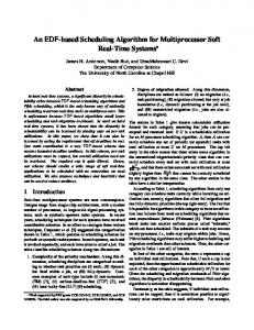
In static scheduling, a program can be represented by a DAG [3] G = (V, E), where V is a set of v nodes and E is a set of directed edges. A node in the DAG represents a task which is a set of instructions that must be executed sequentially without preemption in the same processor. The weight of a node, which represents the amount of time needed for a processor to execute the task, is called the computation cost of the node. The edges in the DAG correspond to the communication messages and precedence constraints among the nodes. The weight of an edge, which represents the amount of time needed to communicate the data, is called the communication cost of the edge. The source node of an edge incident on a node is called a parent of that node. Similarly, the destination node emerged from a node is called a child of that node. A node with no parent is called an entry node and a node with no child is called an exit node. The precedence constraints of a DAG dictate that a node cannot start execution before it gathers all of the messages from its parent nodes. The communication cost among two nodes assigned to the same processor is assumed to be 0. The processors in the target system may be heterogeneous or homogeneous. Heterogeneity of processors means that the processors have different speeds. We assume the processors can be heterogeneous, which means every part of a program can be executed on any processor though the computation time needed on different processors may be different. However, we simply assume the communication links are always homogeneous. The notations used in the paper are summarized in Table 1. Computation costs and communication costs are considered as uncertain variables. Specially, ωk (ni ) denotes uncertain computation cost of node ni on processor k in heterogeneous environments. An example DAG, shown in Fig. 1, will be used as an example later.

20

J. Yang et al.

n1

Z(n1) e12

n2

e17

Z(n2) e26

e15

e14

e13 n3

n4

n5

Z(n3)

Z(n4)

Z(n5)

e27

e38

e48

n6

n7

n8

Z(n6)

Z(n7)

Z(n8)

e69

e79

e89

n9

Z(n9) Fig. 1. Example of a DAG

Table 1. Definitions of Some Notations Symbol ni v p ω(ni ) ωk (ni ) eij c(ni , nj ) P arent(ni ) Child(ni ) x, y x , y t(ni ) l(ni ) F T (ni ) f

Definition Node number of a node in the task graph Number of nodes in the task graph Number of processors in the target system Uncertain computation cost of ni Uncertain computation cost of ni on processor k Directed edge from ni to nj Uncertain communication cost of eij The set of parents of ni The set of children of ni Integer decision vectors Legal integer decision vectors T-level of node ni Legal-order-level of node ni Finish-time of node ni Makespan of a schedule


2.2

21

Computing Top Levels

The top level [3] (t-level ) of a node ni is the length of a longest path (there can be more than one longest path) from an entry node to ni excluding ni . An algorithm for computing the t-levels is shown below. Because computation costs and communication costs are supposed to be stochastic variables in this paper, notations in the algorithm, like ω(ni ) and c(ni , nj ), denote samples of computation costs and communication costs. In the algorithm, t is a vector for storing t-levels. . Construct a list of nodes in topological order. Call it Toplist. . for each node ni in Toplist do . max = 0 . for each node nx ∈ P arent(ni ) do . if t(nx ) + ω(nx ) + c(nx , ni ) > max then . max = t(nx ) + ω(nx ) + c(nx , ni ) . endif . endfor . t(ni ) = max . endfor

3

Scheduling Representation

The scheduling in this paper is represented by Liu’s[4] formulation via two decision vectors [4] x and y, where x = (x1 , x2 , . . . , xv ) is an integer decision vector representing v nodes with 1 ≤ xi ≤ v and xi = xj for all i = j and i, j = 1, 2, . . . , v. That is , the sequence {x1 , x2 , . . . , xv } is a rearrangement of {1, 2, . . . , v}. And y = (y1 , y2 , . . . , yp−1 ) is an integer decision vector with y0 ≡ 0 ≤ y1 ≤ y2 ≤ . . . ≤ yp−1 ≤ v ≡ yp . We note that the schedule is fully determined by the decision vectors x and y in the following way. For each k(1 ≤ k ≤ p), if yk = yk−1 , processor k is not used; if yk > yk−1 , processor k is used and processes nodes nxyk−1 +1 , nxyk−1 +2 , . . . , nxyk in turn. Thus the schedule of all processors is as follows: Processor 1: nxy0 +1 → nxy0 +2 → . . . → nxy1 ; Processor 2: nxy1 +1 → nxy1 +2 → . . . → nxy2 ; ... Processor p: nxyp−1 +1 → nxyp−1 +2 → . . . → nxyp . 3.1

Generating Legal Schedule

For a given random integer decision vectors (x, y), we have to rearrange them to guarantee that the precedence constraints are not violated. For example, if there are precedence relations between two nodes ni and nj , eij ∈ E, and both of them are assigned to the same processor, we should guarantee that ni will

22

J. Yang et al.

be executed before nj . If there are no precedence relations between two nodes, however, they can be executed in any order in that processor. We can get a legal schedule by rearranging the list of nodes within each processor by ascending order of t-levels. However, the t-level ordering condition is only a necessary condition, so the optimal schedule may not satisfy it. To reduce the likelihood of this happening, we define legal-order-levels which is generated from t-levels of nodes. The algorithm to compute legal-order-levels is shown below. In the algorithm, t is a vector of t-levels and l is a vector for storing legal-order-levels. . . . . . . . . .

Construct a list of nodes in topological order. Call it Toplist. for each node ni do Initialize l(ni ) = t(ni ) endfor for each node ni in Toplist do Compute max = max{l(nj )}, nj ∈ P arent(ni ) Compute min = min{l(nj )}, nj ∈ Child(ni ) Generate a random l(ni ) which satisfies min < l(ni ) < max endfor

Finally we can compute legal integer decision vectors (x , y ) by rearranging nodes of the scheduling which is determined by (x, y). The steps are listed as follows. . Compute t-level t(ni ) for each node ni . Compute legal-order-levels l(ni ) for each nodes ni . for each integer k, 1 ≤ k ≤ p do . if yk > yk−1 then . Resort (xyk−1 +1 , xyk−1 +2 , . . . , xyk ) by ascending order of legal-orderlevels . endif . endfor . x = x . y = y 3.2

Stochastic Programming Model

For the multiprocessor scheduling problem, we can consider factors such as throughput, makespan, and processor utilization for the objective function. The objective function used for our algorithm is based on makespan, the overall finish-time of a parallel program. The makespan of a schedule is defined as follows: f (ω, c, x , y ) = max F T (ni ) ni ∈V

(1)

F T (ni ) denotes finishing time of node ni . For a given DAG, the makespan is a function of computation costs ω, communication costs c and the legal schedule (x , y ).


23

In this paper, the makespan of a schedule is also uncertain because all the computation costs and communication costs are given by stochastic variables. We introduce an stochastic expected value model which optimizes the expected makespan subject to some expected constraints. We assume that the expected makespan E[f ] should not exceed the target value b. Thus we have a constraint E[f ] − b = d+ , in which d+ ∨ 0 (the positive deviation) will be minimized. Then, we have the following stochastic expected value model: ⎧ min d+ ∨ 0 ⎪ ⎪ ⎪ ⎪ subject to: ⎪ ⎪ ⎨ E[f (ω, c, x , y )] − b = d+ (2) ω(ni ), ni ∈ V, stochastic variables ⎪ ⎪ ⎪ ⎪ c(ni , nj ), eij ∈ E, stochastic variables ⎪ ⎪ ⎩ (x , y ), legal integer decision vectors In order to compute the uncertain function E[f ], first, a legal schedule (x , y ) is generated from (x, y). Second, we repeat N times to generate ω and c according to their probability measure and use the samples to compute Nfi = f (ω, c, x , y ), i = 1, 2, . . . , N . Finally, the value E[f ] is estimated by N1 i=1 fi provided that N is sufficiently large, which is followed from the strong law of large numbers. Note that other stochastic models such as stochastic chance-constrained model and stochastic dependent-chance model can also be used under different circumstances for modeling different stochastic systems. Stochastic simulations based on those stochastic models will be used. In this paper, without loss of generality, we only discuss the simplest one, stochastic expected value model.

4

Uncertain Intelligent Scheduling Algorithm

In this paper, we present an uncertain intelligent scheduling algorithm based on stochastic simulation and genetic algorithm to solve the stochastic expected value programming problem. From the mathematical viewpoint [4], there is no difference between deterministic mathematical programming and stochastic programming except for the fact that there exist uncertain functions in the latter. If the uncertain functions can be converted to their deterministic forms, we can obtain equivalent deterministic models. However, in general, we cannot do that. It is thus more convenient to deal with them by stochastic simulations. Genetic algorithm is a stochastic search method for optimization problems based on the mechanics of natural selection and natural genetics and it has demonstrated considerable success in providing good solutions to many complex optimization problems. The standard genetic algorithm is shown below. . Generate initial population . while number of generations not exhausted do . for i = 1 to P opulationSize do . Randomly select two chromosomes and crossover

24

J. Yang et al.

. Randomly select one chromosome and mutation . endfor . Evaluate chromosomes and perform selection . endwhile . Report the best chromosome as the final solution The initialization, evaluation, crossover and mutation operations, which are used in our algorithm, are revised as follows. 4.1

Initialization

We encode a schedule into a chromosome (x, y), where x, y are the same as the decision vectors. For the gene section x, we define a sequence {x1 , x2 , . . . , xv } with xi = i, i = 1, 2, . . . , v. In order to get a random rearrangement of {1, 2, . . . , v}, we repeat the following process from j = 1 to v: generating a random position v between j and v, and exchanging the values of xj and xv . For each i with 1 ≤ i ≤ p − 1, we set yi as a random integer between 0 and v. Then we rearrange the sequence {y1 , y2 , . . . , yp−1 } from small to large and thus obtain a gene section y = (y1 , y2 , . . . , yp−1 ). Finally, (x, y) is used to generate and replaced by legal integer decision vectors (x , y ) to guarantee that the produced schedule is legal. In this way, we can ensure that the produced chromosome (x, y) is always feasible. 4.2

Evaluation

Evaluation function is to assign a probability of reproduction to each chromosome so that its likelihood of being selected is proportional to its fitness relative to the other chromosomes in the population. That is, the chromosomes with higher fitness will have more chance to produce offspring by using roulette wheel selection. We define the rank-based evaluation function as a(1 − a)i−1 ,i = 1, 2, . . ., P opulationSize, where a ∈ (0, 1) is a given parameter. Note that i = 1 means the best individual, i = P opulationSize the worst one. 4.3

Crossover

Let us illustrate the crossover operator on the pair (x1 , y1 ) and (x2 , y2 ). First, we generate legal integer decision vectors for (x1 , y2 ) and (x2 , y1 ), which are denoted as (x1 , y2 ) and (x2 , y1 ). Then, two children are produced by the crossover operation as (x1 , y2 ) and (x2 , y1 ). Note that the obtained chromosomes (x1 , y2 ) and (x2 , y1 ) in this way are always feasible. 4.4

Mutation

We mutate the parent (x, y) in the following way. For the gene x, we randomly generate two mutation positions v1 and v2 between 1 and v. If v1 ≤ v2 ,


25

we rearrange the sequence xv1 , xv1 +1 , . . . , xv2 at random to form a new sequence xv1 , xv1 +1 , . . . , xv2 . Else, we rearrange the sequence x1 , x2 , . . . , xv2 −1 , xv1 +1 , xv1 +2 , . . . , xv at random to form two new sequences x1 , x2 , . . . , xv2 −1 and xv1 +1 , xv1 +2 , . . . , xv . Similarly, for the gene y, we generate two random mutation positions v1 and v2 between 1 and p − 1, and set yi as a random integer number yi between 0 and v for i = v1 , v1 + 1, . . . , v2 if v1 ≤ v2 . Or i = 1, 2, . . . , v2 − 1, v1 + 1, v1 + 2, . . . , v if v1 > v2 . We then rearrange the sequence from small to large and obtain a new gene section y. Finally, we generate legal integer decision vectors (x , y ) and replace the parent with the offspring (x , y ).

5

Performance Results

In this section, we use the DAG shown in Figure 1, and assume that the number of processors is 4. Note that the problem is NP-hard even if the variables are constants. So the solution of our algorithm may be near-optimal, as other genetic algorithms. In this section, we focus on the differences between stochastic environments and constant environments. The simulation results show that our algorithm often succeed in finding best schedule that fit more to the real applications from those schedules which are considered the same in other algorithms that use constant computation costs and communication costs. Example 1. In the first example, we assume that processors in target system are homogeneous, and all of the computation costs and communication costs are normally distributed variables, which may fit more than other distributions to real applications. An normally distributed random variable is denoted by N (μ, σ 2 ), where μ and σ are given real numbers. If we use the means of computation costs and communication costs in Table 2 instead of the random variables, we can get schedules produced by several list scheduling algorithms [3] such as dynamic critical path (DCP) algorithm[5], modified critical path (MCP) algorithm[6] and so forth. The schedule generated by the DCP algorithm is shown below,which is an optimal schedule (makespan = 16) under determinate costs assumption. We denote it as DCP-1. Table 2. Normally distributed computation costs and communication costs Symbol Definition ω(1) N (2, 1) ω(4) N (4, 1) ω(7) N (4, 1) c(1, 2) N (4, 1) c(1, 5) N (1, 1) c(2, 7) N (1, 1) c(6, 9) N (5, 1)

Symbol ω(2) ω(5) ω(8) c(1, 3) c(1, 7) c(3, 8) c(7, 9)

Definition N (3, 1) N (5, 1) N (4, 1) N (1, 1) N (10, 1) N (1, 1) N (6, 1)

Symbol ω(3) ω(6) ω(9) c(1, 4) c(2, 6) c(4, 8) c(8, 9)

Definition N (3, 1) N (4, 1) N (1, 1) N (1, 1) N (1, 1) N (1, 1) N (5, 1)

26

J. Yang et al.

Processor Processor Processor Processor

1: 2: 3: 4:

n4 → n8 → n6 → n9 ; n1 → n2 → n7 ; n3 → n5 ; is not used.

Actually there are some more optimal schedules in this problem. Another optimal schedule produced by DCP with different scheduling list [2] is denoted by DCP-2 shown below. Processor Processor Processor Processor

1: 2: 3: 4:

n1 → n2 → n7 ; n4 → n8 → n9 ; n3 → n5 ; n6 .

The schedule produced by MCP algorithm which is not an optimal schedule (makespan = 20) is shown below and denoted by MCP. Processor Processor Processor Processor

1: 2: 3: 4:

n1 → n4 → n2 → n7 → n9 ; n3 → n6 ; n8 ; n5 .

We suppose that the target value of expected makespan is b = 0. A run of the uncertain intelligent scheduling (UIS) algorithm (10000 cycles in stochastic simulation, 400 generations in genetic algorithm) shows that the optimal schedule which is denoted by UIS-1 is Processor 1: n1 → n2 → n7 → n8 → n9 ; Processor 2: n4 → n5 ; 21 UIS−1 UIS−2 UIS−3 DCP−1 DCP−2

20

Expected makespan

19

18

17

16

15

14

0

200

400 600 Number of samples

800

Fig. 2. Expected makespans of example 1

1000


27

Processor 3: n3 ; Processor 4: n6 . Note that the schedules DCP-1, DCP-2 and UIS-1 are all optimal schedules under determinate costs assumption, but they perform differently when costs have uncertainty. In uncertain environment, simulation results show that the expected makespans (10000 samples in simulation) of MCP, DCP-1, DCP-2 and UIS-1 are 20.34, 17.59, 16.97 and 16.41. Example 2. In the second example, one processor in target system is heterogeneous and a little faster than the other three. Without lose of generality, we assume that Processor 1 is a little faster. The computation costs on this processor are listed in Table 3. A run of UIS Algorithm (10000 cycles in stochastic simulation, 400 generations in genetic algorithm) shows that the optimal schedule is Processor Processor Processor Processor

1: 2: 3: 4:

n1 → n2 → n7 → n8 → n9 ; n3 → n5 ; n4 ; n6 .

We denote the schedule as UIS-2. The 4 schedules in the former example are also used in simulation. To guarantee that the best schedule is obtained, we suppose that the processor to which most nodes are assigned is the faster one. In uncertain environment, simulation results show that the expected makespans (10000 samples in simulation) of MCP, DCP-1, DCP-2 ,UIS-1 and UIS-2 are 19.11, 16.91, 15.76, 15.39 and 15.32.

20 UIS−1 UIS−2 UIS−3 DCP−1 DCP−2

19

Expected makespan

18

17

16

15

14

13

0

200


800


1000

28

J. Yang et al. Table 3. Computation costs on Processor 1 in heterogeneous system Symbol Definition ω1 (1) N (1.5, 1) ω1 (4) N (3.5, 1) ω1 (7) N (3.5, 1)

Symbol ω1 (2) ω1 (5) ω1 (8)

Definition N (2.5, 1) N (4.5, 1) N (3.5, 1)

Symbol ω1 (3) ω1 (6) ω1 (9)

Definition N (2.5, 1) N (3.5, 1) N (1, 1)

Example 3. In the third example, we also use the heterogeneous system in the second example. But all the real numbers σ 2 in N (μ, σ 2 ) are changed from 1 to 0.5. A run of UIS Algorithm (10000 cycles in stochastic simulation, 400 generations in genetic algorithm) shows that the optimal schedule is Processor Processor Processor Processor

1: 2: 3: 4:

n1 → n2 → n7 → n5 ; n6 → n8 → n9 ; n4 ; n3 .

We denote the schedule as UIS-3. In uncertain environment, simulation results show that the expected makespans (10000 samples in simulation) of MCP, DCP1, DCP-2 ,UIS-1, UIS-2 and UIS-3 are 18.58, 16.23, 15.24, 15.04, 15.02 and 14.77. The results of the three examples are listed in Table 4. We can see that MCP performs poor because the schedule is not optimal even in the constant costs assumption. However, the other 5 schedules are all optimal (makespan=16) in the case that the costs are constant. They performs differently in uncertain environments. Part of the results are shown in Fig. 2, Fig. 3 and Fig. 4. The curves show the first 1000 samples in the simulation results and MCP is not 17.5 UIS−1 UIS−2 UIS−3 DCP−1 DCP−2

17

Expected makespan

16.5 16 15.5 15 14.5 14 13.5 13

0

200


800


1000


29

Table 4. Simulation Results (10000 samples in simulation) Example System σ 2 MCP 1 homogeneous 1 20.34 heterogeneous 1 19.11 2 heterogeneous 0.5 18.58 3

DCP-1 17.59 16.91 16.24

DCP-2 16.97 15.76 15.24

UIS-1 UIS-2 UIS-3 16.41 16.45 16.66 15.39 15.32 15.42 15.04 15.02 14.77

included because the schedule is not optimal even in the case that the costs are constant.

6

Conclusions

In this paper, we present an uncertain intelligent scheduling algorithm to solve the multiprocessor scheduling problem in uncertain environments. We introduce an expected value model based on stochastic simulation and devise a genetic algorithm to obtain optimal solution. In simulation examples, it shows that our algorithm performs better than other algorithms in uncertain environments.

References 1. Hou, E.S.H.: A genetic algorithm for multiprocessor scheduling. IEEE Transaction on Parallel and Distributed Systems 5(2), 113–120 (1994) 2. Kwok, Y.K., Ahmad, I.: Efficient scheduling of arbitrary task graphs to multiprocessors using a parallel genetic algorithm. Journal of Parallel and Distributed Computing (47), 58–77 (1997) 3. Kwok, Y.K., Ahmad, I.: Static scheduling algorithms for allocating directed task graphs to multiprocessors. ACM Computing Surveys 31(4), 406–471 (1999) 4. Liu, B.: Theory and Practice of Uncertain Programming, 1st edn. Physica-Verlag, Heidelberg (2002) 5. Kwok, Y.K., Ahmad, I.: Dynamic critical-path scheduling: An effective technique for allocating task graphs to multiprocessors. IEEE Tran. Parallel Distrib. Syst. 7(5), 506–521 (1996) 6. Wu, Gajaki: Hypertool: A programming aid for message-passing systems. IEEE Trans. Parallel Distrib. Syst. 1(3), 330–343 (1990)