function of the algorithm performing the mapping and scheduling under strict ..... in Section IV-C. The optimization system was written with Python language.
Hybrid Algorithm for Mapping Static Task Graphs on Multiprocessor SoCs Heikki Orsila, Tero Kangas, and Timo D. H¨am¨al¨ainen Institute of Digital and Computer Systems Tampere University of Technology P.O. Box 553, 33101 Tampere, Finland Email: {heikki.orsila, tero.kangas, timo.d.hamalainen}@tut.fi Abstract— Mapping of applications on multiprocessor Systemon-Chip is a crucial step in the system design to optimize the performance, energy and memory constraints at the same time. The problem is formulated as finding solutions to an objective function of the algorithm performing the mapping and scheduling under strict constraints. Our solution is a new hybrid algorithm that distributes the computational tasks modeled as static acyclic task graphs The algorithm uses simulated annealing and group migration algorithms consecutively and it combines a non-greedy global and greedy local optimization techniques to have good properties of both ways. The algorithm begins as coarse grain optimization and moves towards fine grained optimization. As a case study we used ten 50-node graphs from the Standard Task Graph Set and averaged results over 100 optimization runs. The hybrid algorithm gives 8% better execution time on a system with four processing elements compared to simulated annealing. In addition, the number of iterations increased only moderately, which justifies the new algorithm in SoC design.
I. I NTRODUCTION Contemporary embedded system applications demand increasing computing power and reduced energy consumption at the same time. Multiprocessor System-on-Chip implementations have become more popular since it is often more reasonable to use several low clock rate processors than a single high-performance one. In addition, the overall performance can be increased by distributing processing on several microprocessors raising the level of parallelism. However, efficient multiprocessor SoC implementation requires exploration to find an optimal architecture as well as mapping and scheduling of the application on the architecture. This, in turn, calls for optimization algorithms in which the cost function consists of execution time, communication time, memory, energy consumption and silicon area constraints, for example. The optimal result is obtained in a number of iterations, which should be minimized to make the optimization itself feasible. One iteration round consists of application task mapping, scheduling and as a result of that, evaluation of the cost function. In a large system this can take even days. The principal problem is that in general the mapping of an application onto a multiprocessor system is an NP-problem. Thus verifying that any given solution is an optimum needs exponential time and/or space from the optimization algorithm. Fortunately it is possible in practice to device heuristics that can reach near optimal results in polynomial time and space for common applications.
We model the SoC applications as static acyclic task graphs (STGs) in this papers. Distributing STGs to speedup the execution time is a well researched subject [1], but multiprocessors SoC architectures represent a new problem domain with significantly more requirements compared to traditional multiprocessor systems. This paper presents a new algorithm especially targeted to map and schedule applications for multiprocessor SoCs in an optimal way. In this paper the target is to optimize the execution time, but the algorithm is also capable of optimizing memory and energy consumption compared to previous proposals. The hybrid algorithm applies a non-greedy global optimization technique known as simulated annealing (SA) and a greedy local optimization technique known as the group migration (GM) algorithm. The basic concepts and the related work of task parallelization, SA and GM are presented in Section II. The contribution of this paper is the hybrid task mapping algorithm, which is described in Section III. The algorithm was evaluated with a set of task graphs and compared to the pure SA algorithm as reported in Section IV. Finally, the concluding remarks are given.
II. R ELATED W ORK Wild et. al considered simulated annealing and tabu search for SoC application parallelization [2]. Their algorithm uses a special critical path method to identify important tasks that need to be relocated. Also, Vahid [3] considered prepartitioning to shrink optimization search space, and in addition they apply various clustering algorithms, such as group migration algorithm, to speedup the execution time. This is similar approach to us, in which we enhance simulated annealing with the group migration. Lei et al. [4] considered a two-step genetic algorithm for mapping SoC applications to speedup the execution time. Their approach starts with coarse grain optimizations and continues with fine grain optimizations as in our approach. Compared to our algorithm, they have stochastic algorithms in both steps. Our algorithm adds more reliability as the second step is deterministic.
A (1)
D (4)
1
B (2) 2
1 1
E (5)
1
F (6)
4 C (3)
Fig. 1. An example STG with computational costs in nodes and communication costs at edges. Node F is the result node that is data dependent on all other nodes
A. Static Task Graphs Nodes of the STG are finite deterministic computational tasks, and edges represent data dependencies between the nodes. Computational nodes block until their data dependencies are resolved. Node weights represent the amount of computation associated with a node. Edge weights represent amount of communication needed to transfer results between the nodes. Fig. 1 shows an STG example. Node F is the result node which is data dependent on all other nodes. Nodes A, C and D are nodes without data dependencies, and hence they are initially ready to run. Each node is mapped to a specific processing element in the SoC. The STG is fully deterministic, meaning that the complexity of the computational task is known in advance, and thus no load balancing technique, such as task migration, is not needed. The distribution is done at compile time, and the run-time is deterministic. When a processing element has been chosen for a node it is necessary to schedule the STG on the system. Schedule determines execution order and timing of execution for each processing element. The scheduler has to take into account the delays associated with nodes and edges, and data dependencies which affect the execution order. B. Simulated Annealing SA is a probabilistic non-greedy algorithm [5] that explores search space of a problem by annealing from a high to a low temperature state. The greediness of the algorithm increases as the temperature decreases, being almost greedy at the end of annealing. The algorithm always accepts a move into a better state, but also into a worse state with a changing probability. This probability decreases along with the temperature, and thus the algorithm becomes greedier. The algorithm terminates when the maximum number of iterations have been made, or too many consecutive moves have been rejected. Fig. 2 shows the pseudo-code of the SA algorithm used in the hybrid algorithm. Implementation specific issues compared to the original algorithm are mentioned in Section IV-A. The Cost function evaluates badness of a specific mapping by calling the scheduler to determine execution time. S0 is the initial state of the system, and T0 is the initial temperature. Temperature–Cooling function computes a new temperature as a function of initial temperature T0 and iteration i. Move function makes a random move to another state. Random function returns a random value from the interval [0, 1). Prob
S IMULATED -A NNEALING(S0 , T0 ) 1 S ← S0 2 C ← C OST(S0 ) 3 Sbest ← S 4 Cbest ← C 5 Rejects ← 0 6 for i ← 1 to imax 7 do T ← T EMPERATURE -C OOLING(T0 , i) 8 Snew ← M OVE(S, T ) 9 Cnew ← C OST(Snew ) 10 r ← R ANDOM() 11 p ← P ROB(Cnew − C, T ) 12 if Cnew < C or r < p 13 then if Cnew < Cbest 14 then Sbest ← Snew 15 Cbest ← Cnew 16 S ← Snew 17 C ← Cnew 18 Rejects ← 0 19 else Rejects ← Rejects + 1 20 if Rejects ≥ Rejectsmax 21 then break 22 return Sbest Fig. 2.
Pseudo-code of the simulated annealing algorithm
function computes a probability that a move that increases the cost is accepted. C. Group Migration Algorithm Group migration algorithm ([3], [6]) is a greedy local search technique that changes mapping of STG nodes one by one, accepting only moves that improve current solution as determined by the scheduler. Fig. 3 shows pseudo-code of the GM algorithm used in the hybrid algorithm. The function Group–Migration calls the function GM–Round as long as the solution improves. Function GM–Round tries to move each task one by one from its PE to all other PEs. If it finds a move that decreases cost, it records the change, and restores the original mapping and goes to the next task. After all tasks have been tried, it takes the best individual move, applies that move on the mapping, and marks the associated task as non-movable. Any task that has been marked non-movable will not be considered as a movable candidate again. Then the algorithm starts from the beginning, trying each movable task again. This is continued until no cost decrease is found. III. T HE P ROPOSED H YBRID A LGORITHM A. Mapping The hybrid algorithm presented in this paper uses SA and GM algorithms to support each other. Fig. 4 shows pseudocode of the main optimization loop. Initially the mapping is set by the function Fast–Premapping shown in Fig. 5. Fast premapping distributes node mappings so that parents of a
G ROUP -M IGRATION(S) 1 while T rue 2 do Snew ← GM-ROUND(S) 3 if C OST(Snew ) < C OST(S) 4 then S ← Snew 5 else break 6 return S GM-ROUND(S0 ) 1 S ← S0 2 Mcost ← C OST(S) 3 M oved ← [F alse] ∗ Ntasks 4 for i ← 1 to Ntasks 5 do Mtask = NIL 6 MP E = NIL 7 for t ← 0 to Ntasks − 1 8 do if M oved[t] = T rue 9 then continue 10 Sold ← S 11 for A ← 0 to NP Es − 1 12 do if A = Aold 13 then continue 14 S[t] ← A 15 if C OST(S) < Mcost 16 then continue 17 Mcost = C OST(S) 18 Mtask = t 19 Magent = A 20 S ← Sold 21 if Magent = NIL 22 then break 23 M oved[Mtask ] ← T rue 24 S[Mtask ] ← Magent 25 return S Fig. 3.
Pseudo-code of the group migration algorithm
child are on different PEs. As an example, nodes in the Fig. 1 would be premapped to 3 PE system as follows: F 7→ P E 1, B 7→ 1, E 7→ 2, C 7→ 3, A 7→ 1, and D 7→ 2. SA and GM algorithms are called sequentially until the optimization terminates. There are two specialties in this approach. First, SA is called many times, but with each time the initial temperature is half of that of the previous iteration. The SA algorithm itself can visit a good state but leave it for a worse state with certain probability, since the algorithm is not totally greedy. To overcome this deficiency our SA implementation returns the best state visited from any SA algorithm invocation, and the next call of SA begins from the best known state. Furthermore, since initial temperature is halved after each invocation, the algorithm becomes greedier during the optimization process. This process is iterated until a final temperature Tf inal has been reached. This enables both fine and coarse grain search of the state space with reasonable optimization cost. At each invocation it becomes harder for
O PTIMIZATION() 1 S ← FAST-P REMAPPING() 2 T ← 1.0 3 while T > Tf inal 4 do S ← S IMULATED -A NNEALING(S, T ) 5 if U seGroupM igration = T rue 6 then S ← G ROUP -M IGRATION(S) 7 T ← T2 8 return S Fig. 4.
Pseudo-code of the main optimization loop
FAST-P REMAPPING() 1 Assigned ← [F alse] ∗ Ntasks 2 S ← [NIL] ∗ Ntasks 3 S[ExitN ode] ← 0 4 F ← EmptyF if o 5 F IFO -P USH(F, ExitN ode) 6 while F 6= EmptyF if o 7 do n ← F IFO -P ULL(F ) 8 A ← S[node] 9 for each parent p of node n 10 do if Assigned[p] = T rue 11 then continue 12 Assigned[p] = T rue 13 S[p] = A 14 F IFO -P USH(F, p) 15 A ← (A + 1) mod Nagents 16 return S Fig. 5.
Pseudo-code of the fast premapping algorithm
the algorithm to make drastic jumps in the state space. B. Scheduling This paper considers node weights in task graphs as execution time to perform computation on a processing element and edge weights as time to transfer data between PEs in a SoC communication network. The scheduler used in this system is a B-level scheduler [1]. Since nodes are mapped before scheduling, B-level priorities associated with the nodes remain constant during the scheduling. This approach accelerates optimization, because B-level priorities need not to be recalculated. There exists better scheduling algorithms in the sense that they produce shorter schedules, but they are more expensive in optimization time [7]. When scheduling is finished the total execution time of the STG is known, and thus the cost of the mapping can be evaluated. IV. R ESULTS A. Case Study Arrangements The case study experiment used 10 random graphs, each having 50 nodes, from the Standard Task Graph set [8]. We used random graphs to evaluate optimization algorithms as
Optimization progress
−4
3
x 10
2.9
2.8
Cost
2.7
2.6
2.5
2.4 SA invocations 2.3
0
2000
4000
Best
6000 8000 Iteration
10000
12000
14000
Fig. 6. Simulated annealing of a 50 node random STG. Cost function is the execution time for executing the mapped graph on two processing elements Optimization progress
−4
3
x 10
2.9
2.8
2.7 Cost
fairly as possible. Non-random applications may well be relevant for common applications, but they are dangerously biased for mapping algorithm comparison. Investigating algorithm bias and classifying computational tasks based on bias are not topics in this paper. Random graphs have the property to be neutral of the application, and thus mapping algorithms that do well on random graphs will do well on average applications. Optimization was run 10 times independently for each task graph. Thus 100 optimization runs were executed for both algorithms. The objective function for optimization was the execution time of a mapped task graph. The random graphs did not have exploitable parallelism for more than 4 PEs so that was chosen as the maximum number of PEs for the experiment. Thus speedup of mapped task graphs was obtained for 2, 3, and 4 PEs. The SoC was a message passing system where each PE had some local memory, but no shared memory. The PEs were interconnected with a single dynamically arbitrated shared bus that limits the SoC performance because of bus contention. The optimizations were executed on a 10 machine Gentoo Linux cluster. Optimization runs were distributed by using rsync to copy input and output files between machines and SSH to execute shell scripts remotely. Initially one machine uploaded input files and optimization software to all machines, and then commanded each machine to start optimization software. After optimization was finished on all machines, the results were downloaded back. All machines were 2.8 GHz Intel Pentium 4 machines with 1 GiB of memory. Execution time for optimization is given in Section IV-C. The optimization system was written with Python language. It is an object-oriented dynamically typed language that is interpreted during execution. Python language was chosen to save development time with object-oriented high-level techniques. The optimization system code is highly modular in object-oriented fashion. The implementation of simulated annealing algorithm has the following specific issues. Temperature–Cooling function shown in Fig. 2. computes a new temperature with formula T0 ∗ pi , where p is the percentage of temperature preserved on each iteration. Move function makes a random state change so that Ntasks T0 random tasks are moved separately to a random PE, where Ntasks is the number of tasks in the task graph. Prob function is 1 , Prob(∆C, T ) = ∆C ) 1 + exp( 0.5C 0T
2.6
2.5
2.4
2.3
GM
GM
GM 0
2000
4000
6000 Iteration
8000
Best 10000
12000
Fig. 7. Simulated annealing combined with group migration algorithm of a 50 node random STG
where C0 = Cost(S0 ). The C0 term is a special normalization factor chosen to make annealing parameters more compatible with different graphs.
is decelerated between each call. The first downfall is the largest, and after that downfalls are less drastic. Second, SA and GM are used to complement each other. SA can climb from a local minima to reach a global minimum. SA does not search for local minima, so it does not exploit local similarity to reach better states by exploring local neighborhoods. The GM algorithm is used to locally optimize SA solutions as far as possible. Fig. 7 shows progress of combined SA and GM optimization. At around iteration 2250 the GM algorithm is able find a locally better solution and thus the objective function value decreases. SA might not have found that solution. At around iteration 8300 GM finds the best solution by local optimization.
B. SA and GM Iterations
C. Hybrid Algorithm
Fig. 6 shows the progress of annealing without the group migration algorithm for a random 50-node STG. The cost function is the execution time for executing the mapped graph on two processing elements. This figure shows how each invocation of SA improves the overall solution, but improving
The hybrid algorithm was compared with pure simulated annealing by obtaining speedups for parallelized task graphs. Speedup is defined as to /tp , where to is the original execution time of the mapped graph and tp is the parallelized execution time.
TABLE I AVERAGED SPEEDUPS AND NUMBER OF COST FUNCTION EVALUATIONS
3 2 PEs 3 PEs 4 PEs
FOR ALGORITHMS
SA speedup Hybrid speedup Difference-% SA cost evaluations Hybrid cost evaluations Evaluations difference-%
2 PEs 1.467 1.488 1.4 1298k 1313k 3.6
3 PEs 1.901 1.977 4.0 857k 1047k 14.9
4 PEs 2.103 2.278 8.3 767k 1322k 34.5
Execution time speedup
2.5
2
1.5
1
0.5 3
2.5
Execution time speedup
0
2 PEs 3 PEs 4 PEs
1
2
3
4
5
6 7 Task graph
8
9
10
Fig. 9. Per task graph speedups for the hybrid algorithm with 2, 3, and 4 processing elements
2
1.5
1
0.5
0
1
2
3
4
5
6 7 Task graph
8
9
10
Fig. 8. Per task graph speedups for SA algorithm with 2, 3, and 4 processing elements
The results are shown in Table I. The advantage of the hybrid algorithm increases as the number of PEs increases. With 2 PEs, the benefit is small, but with 3 PEs it is 4.0% better speedup on average for 10 graphs with 10 independent runs. With 4 PEs the benefit is 8.3% better speedup (0.175 speedup units). However, greater speedup is achieved with the cost of optimization time. Fig. 8 shows speedup values for each graph when SA algorithm was used for optimization. There is 10 bar sets in the figure, and each bar set presents 3 values for 2, 3, and 4 processing elements respectively. All values are averaged over 10 independent runs. Fig. 9 shows same values for the hybrid algorithm. Optimization time is determined by the number of cost function evaluations as tabulated in Table I. The hybrid algorithm has 3.6%, 14.9%, and 34.5% more cost function evaluations for 2, 3, and 4 PEs respectively. Total running time for optimizations was 40036 seconds for SA, and 62007 seconds for the hybrid algorithm. Thus hybrid algorithm ran 55% longer in wall time. Compared to other proposals [2], the average improvement of 8% is considered very good. V. C ONCLUSION The new method applies both local and global optimization techniques to speedup execution time of static task graphs. The new method is a hybrid algorithm that combines simulated annealing and group migration algorithms in a novel fashion.
The algorithm takes advantage of both greedy and non-greedy optimization techniques. Pure simulated annealing and the hybrid algorithm were compared. The results show 8.3% speedup increase for the hybrid algorithm with 4 PEs averaged over 100 test runs with the expense of 34.5% iteration rounds. Further research is needed to investigate simulated annealing heuristics that explore new states in the mapping space. A good choice of mapping heuristics can improve solutions and accelerate convergence, and it is easily applied into the existing system. Further research should also investigate how this method applies to optimizing other factors in a SoC. Execution time is one factor, and memory and power consumption are others. R EFERENCES [1] Y.-K. Kwok and I. Ahmad, Static scheduling algorithms for allocating directed task graphs to multiprocessors, ACM Comput. Surv., Vol. 31, No. 4, pp. 406-471, 1999. [2] T. Wild, W. Brunnbauer, J. Foag, and N. Pazos, Mapping and scheduling for architecture exploration of networking SoCs, Proc. 16th Int. Conference on VLSI Design, 2003. [3] F. Vahid, Partitioning sequential programs for CAD using a threestep approach, ACM Transactions on Design Automation of Electronic Systems, Vol. 7, No. 3, pp. 413-429, 2002. [4] T. Lei and S. Kumar, A two-step genetic algorithm for mapping task graphs to a network on chip architecture, Proceedings of the Euromicro Symposium on Digital System Design (DSD’03), 2003. [5] S. Kirkpatrick, C. D. Gelatt Jr., and M. P. Vecchi, Optimization by simulated annealing, Science, Vol. 200, No. 4598, pp. 671-680, 1983. [6] D. D. Gajski, F. Vahid, S. Narayan, and J. Gong, Specification and design of embedded systems, Pearson Education, 1994. [7] I. Ahmad and Y.-K. Kwok, Analysis, evaluation, and comparison of algorithms for scheduling task graphs on parallel processors, Parallel Architectures, Algorithms, and Networks, 1996. [8] Standard task graph set, http://www.kasahara.elec.waseda.ac.jp/schedule, 2003.