EMail: {mni | reich } @cse.unl.edu. ABSTRACT. Comprehensive two-dimensional gas chromatography (GCxGC) is an emerging technology for chemical ...
A STATISTICS-GUIDED PROGRESSIVE RAST ALGORITHM FOR PEAK TEMPLATE MATCHING IN GCXGC Mingtian Ni and Stephen E. Reichenbach ∗ Department of Computer Science and Engineering University of Nebraska - Lincoln Lincoln, NE 68588-0115, USA EMail: {mni | reich } @cse.unl.edu ABSTRACT
Two types of information are associated with template peaks: computed features (peak location, area, volume, shape, etc) and annotated information (chemical names, chemical group names, etc). Typically, only computed features are used for matching. In this paper, we consider peak location (the coordinates of the pixel with the largest value within the peak) as the primary feature for matching. In such a case, the peak template matching problem becomes a point pattern matching problem. The problem is formalized as follows: Given point template (template point set) n P = {pi (xi , yi )}m i=1 , target point set Q = {qi (ui , vi )}i=1 , and a transformation space T , find a transformation t in T that maximizes the number of points in P that can be matched with points in Q.
Comprehensive two-dimensional gas chromatography (GCxGC) is an emerging technology for chemical separation. Chemical identification is one of the critical tasks in GCxGC analysis. Peak template matching is a technique for automatic chemical identification. Peak template matching can be formulated as a point pattern matching problem. This paper proposes a progressive RAST algorithm to solve the problem. Search space pruning techniques based on peak location distributions and transformation distributions are also investigated for guided search. Experiments on seven real data sets indicate that the new techniques are effective. 1. PEAK TEMPLATE MATCHING FOR GCXGC
2. RECOGNITION BY ADAPTIVE SUBDIVISIONS OF TRANSFORMATION SPACE
Comprehensive two-dimensional gas chromatography (GCxGC) is an emerging technology for chemical separation that provides an order-of-magnitude increase in separation capacity over traditional GC [1]. Given a chemical sample, the output data of GCxGC can be represented, visualized, and processed as an image. In the image, each resolved chemical substance produces a small peak or cluster of pixels with values that are larger than the background values. The objective of GCxGC analysis is to produce an accurate report on the observed chemicals and their quantity in a sample. The major image analysis tasks include:
A wide variety of techniques have been developed for solving point pattern matching problems, including searching matching space [2], alignment [3], Hough transforms [4], geometric hashing (also called pose clustering) [5], minimizing Hausdorff distance [6, 7], computational geometry [8], etc. Recognition by Adaptive Subdivision of Transformation Space (RAST) is another family of algorithms [9, 10]. The fundamental idea of RAST is hierarchical searching for a globally optimal solution in the transformation space. With RAST, each pair of a template point and a target point defines a constraint set (a region) in the transformation space, containing the transformations that can match the two points within some distance tolerance. Two constraint sets are called compatible if their template points are different. To find a transformation that matches k template points, RAST finds a point in transformation space where k compatible constraint sets overlap. RAST starts with some initial region (usually rectangular) in the transformation space, and computes which of the O(mn) constraint sets intersect the region. If enough compatible ones do, it then subdivides the region and repeats the calculation on each of the subregions. Otherwise, it rejects the region. The algorithm accepts a region if it intersects enough constraint sets and its size is smaller than some preset threshold. The information about the transformation space is implicitly hard-coded in RAST algorithms. This paper uses constrained global affine transformations. The constrained global affine transformation from p(xp , yp ) to q(uq , vq ) is: · ¸ · ¸· ¸ · ¸ uq sx hx (= 0.0) xp tx = + vq hy sy yp ty
1. Separating individual peaks from background, 2. Quantifying each peak, and 3. Identifying the chemicals for peaks of interest. GCxGC images contain potentially thousands of peaks in complex patterns, making chemical identification a challenging problem. Manual identification of chemicals is tedious and timeconsuming. An alternative is to use peak template matching. A peak template is a set of peaks with known chemical names and other characteristics (e.g., whether a chemical is an internal standard). Simple templates are created through interactive annotation. Template matching tries to establish as many correspondences as possible from peaks in the template to peaks in the target peak set. After correspondences are established, the information (e.g., chemical name) carried by the peaks in the template is copied into the corresponding peaks in the target peak set. Consequently, all the matched chemicals in the target peak set are identified. ∗ This material is based upon work supported by the National Science Foundation under Grant No. 0231746.
0-7803-7997-7/03/$17.00 © 2003 IEEE
369
1 if (M (Rs) ≥ kl ) 2 Initialize the priority queue to Rs ; 3 else 4 Finish the search; 5 while ( the priority queue is not empty ) { 6 Extract the first region R; 7 if (R has the desired accuracy) { 8 Report R and M (R) to the user; 9 Check the user’s action for possible termination; 10 if (M (R) < kh ) { 11 Set kl to M (R); 12 Delete from the priority queue those regions whose M (R) ≤ kl ; 13 } 14 else { 15 Finish the search; 16 } 17 } 18 else { 19 Subdivide R into two subregions R1 and R2 ; 20 for ( Ri , i = 1, 2 ) { 21 Compute M (Ri ); 22 if (M (Ri) ≥ kl ) { 23 Enqueue Ri with its priority; 24 } 25 } 26 } 27 }
and hx is set to 0.0, noting that x coordinates are independent of the y coordinates in GCxGC images. The inputs to the basic RAST algorithm are point template P , target point set Q, the number of template points to be matched k, distance tolerance ², and transformation space Rs . Upon termination, the algorithm returns either a constraint set or null. If a constraint set is returned, then some point (transformation) in the constraint set is taken as the solution. Roughly speaking, under such a transformation, there is a subset P ⊆ P of size k such that each point in P lies in the neighborhood of some point in Q, i.e., a part of P is matched to a part of Q. This method has two important properties: • It does not require one to specify in advance which subset of P is to be matched. The subset is found by searching through all possible combinations of points in P . • It does not prevent many-to-one mapping because two compatible constraint sets may have the same target point. In GCxGC, other computed features such as peak volume can be used to break the tie when many-to-one mappings happen. The techniques of minimizing Hausdorff distances also have such properties when partial directed Hausdorff distance is used [6]. While the worst case running time of RAST is exponential in the problem size, the average case running time is polynomial [9]. Compared to the methods of alignment, Hough transforms, and geometric hashing, RAST is slower but provides more reliable solutions [10]. 3. A PROGRESSIVE RAST ALGORITHM
Fig. 1. The Progressive RAST Algorithm.
Given a set of inputs, RAST returns either a constraint set that meets the requirement or null. This scheme does not work well for interactive processing such as in GCImageT M [11]. For interactive applications, users have special concerns: • Prompt responses. Usually, a quick response with a preliminary matching is preferred to a long wait for a possibly better matching. • Range of matched point numbers. It is difficult to determine how many template points will be matched. It becomes easier if RAST takes a range of numbers [kl , kh ], where kl specifies the minimum number of matched points that are expected, and the algorithm stops searching if no less than kh matching points have been found. • Interactive control over the matching process. When the users see enough matched points, they may choose to terminate the process (interacting with the application through a separate event thread). The following progressive RAST algorithm (PRAST) satisfies these requirements. The algorithm extends the non-progressive algorithm proposed by Breuel [9, 10]. The PRAST algorithm progressively reports better matching results and allows the users to terminate the searching at any time. Let M (R) be the number of compatible constraint sets intersecting region R. M (R) gives the upper bound of the number of template points that can be matched by the transformations in R. In the following algorithm description, if R is small enough, M (R) is roughly taken as the number of matched template points (and the matching verifying step is skipped for simplicity). Let [kl , kh ] be the range of the number of template points to be matched. The PRAST algorithm is shown in Figure 1.
The priorities of regions are compared based on two rules: • Smaller regions have higher priorities. This rule forces depth-first searching. • If two regions have the same size, the region with larger M (R) has higher priority. This rule makes the algorithm search first the regions that intersect more constraint sets. The space complexity of PRAST is same as the original version. Let C(kl , kh ) be the computation needed for range [kl , kh ] when PRAST is used and C(k) be the computation needed for k Pkh when RAST is used. It is clear that C(kl , kh ) ≤ k=kl C(k). In practice, because subdivisions are reused during the progressive Pkh search, C(kl , kh ) < k=kl C(k). Based on seven real data sets, Table 1 shows an average 26.5% improvement of PRAST over RAST in time complexity, where: P|P | I(1, |P |) =
k=1
C(k) − C(1, |P |) . P|P | k=1 C(k)
4. PRUNING CONSTRAINT SETS WITH PEAK LOCATION DISTRIBUTION For general object recognition problems in computer vision, objects can take any pose in the images. Consequently, absolute point location is usually not used for recognition directly. For GCxGC, however, peak location encodes the most important information.
370
Table 1. Time complexity of PRAST with comparison to RAST Data set Number of Number of se- I(1, |P |) images lected peaks D2287 sdalk 3 15 2.3% D2287 sdgas 3 580 61% Doixin 3 26 16.7% GCC2002 12 14 10.5% Linearity 5 18 20% NYSDH 5 10 50% PCB 4 17 25%
Under well-controlled conditions, a chemical peak can appear only at slightly different locations from image to image. This property motivates the use of peak location distribution for pruning the constraint sets. The pruning process consists of two steps: 1. Estimating peak location distribution. Let D be a training data set containing several images (peak sets) generated from the same chemical sample or from related samples with the same chemicals. Selected peaks in D are annotated and correspondences are established. For each set of corresponding peaks, the variation is modelled by an uncorrelated normal distribution N (µ, Σ), where µ is the mean vector and Σ is the covariance matrix. Values of µ and Σ are estimated with common techniques such as those in [12]. Upon completion, there is a set of normal distributions {Ni (µi , Σi )}gi=1 with Ni defined at location µi . Subdivide the domain of the peak sets in D using the technique described in Section 5 and save the subdivision for later use.
Fig. 2. Neighborhoods of some peaks in data set D2887 sdgas.
• the regions do not intersect with each other, and • the union of the regions equals to the point set domain. The domain subdivision described here is based on Delaunay triangulation [13]. However, since the triangulation only covers the convex hull of the point set (Figure 3 (a)), some measure must be taken to cover the remaining area. In this investigation, an edge projection technique is used to expand the triangulation (Figure 3 (b)). Given a point set, the O(n2 ) subdivision algorithm runs as follows:
2. Pruning the constraint sets. When preparing the constraint sets for a point p in P , instead of pairing it with every q in Q, only points in the set {q ∈ Q, q ∈ A | P (A | p) ≥ probability threshold} are considered, where A is some neighborhood of p and P (A | p) is the probability that p’s corresponding points lie in A. A is estimated as follows:
1. Raise the input point set into 3D space such that (x, y) is mapped to (x, y, x2 + y 2 ). 2. Use the incremental algorithm to construct the convex hull of the 3D point set [13]. The implementation is based on half-edge data structure and Euler operators [14].
(a) If p is close to some µi , then set p’s distribution to Ni (µi , Σi ). Otherwise, calculate p’s distribution by interpolation (or extrapolation) based on the subdivision computed in the previous step.
3. Project all faces (3D triangles) of the convex hull which face down (negative z direction) back onto the xy plane. The result is the Delaunay triangulation of the original 2D point set.
(b) Use p’s distribution to estimate region A. Figure 2 gives the rectangular neighborhoods of some peaks in data set D2887 sdgas with probability threshold being 99%.
4. Project all the outside edges of the triangulation onto the point set domain boundary along the bisectors of neighboring outside edges. After the projection, outside triangles become polygons. The triangulation is expanded to be a domain subdivision.
Experiments show that the number of candidate points for p decreases from thousands (the entire target point set) to tens by using the pruning technique.
An example of the domain subdivision is given in Figure 3.
5. POINT SET DOMAIN SUBDIVISION
6. ESTIMATING RS WITH TRANSFORMATION DISTRIBUTION
Let (width, height) be the size of an image. Then, [0, width] × [0, height] is defined as the domain of the image as well as the point sets extracted from it. When a domain is subdivided into small regions, the subdivision should meet the following two requirements:
Given the model of global constrained affine transformation, the complexity of finding a matching is primarily determined by the ranges that the transformation parameters vary. If all five parameters vary freely, searching for a solution is expensive. However, experiments show that the optimal transformations for matching
371
acteristics are explored and used for accelerating the search in the RAST algorithm. This paper also proposes a progressive RAST algorithm for interactive applications. Future work includes statistical analysis of spatial configurations of peaks across images and incorporating this knowledge with the local peak location distribution to facilitate the search. 8. REFERENCES
(a)
[1] W. Bertsch, “Two-dimensional gas chromatography, concepts, instrumentation, and applications — Part 2: Comprehensive two-dimensional gas chromatography,” Journal of High Resolution Chromatography, vol. 23, no. 3, pp. 167– 181, 2000.
(b)
[2] H.S. Baird, Model-based Image Matching using Location, MIT Press, Cambridge, MA, 1985.
Fig. 3. (a) Delaunay triangulation. (b) Point set domain subdivision by edge projection.
[3] D. P. Huttenlocher and S. Ullman, “Object recognition using alignment,” in Proc. International Conference on Computer Vision, 1987, pp. 102–111.
GCxGC peak sets are clustered in the transformation space. Consequently, a search over a small region typically will find a good matching. For each training data set, optimal transformations are computed from each peak set to every other peak set, based on leastsquares estimation. A normal distribution N (µ, Σ) is then fit to the distribution of the resultant transformations using common techniques such as those in [12]. Rs is set to be a rectangular region A in the transformation space, where Z N (µ, Σ)dt ≥ certain probability threshold
[4] J. Illingworth and J. Kittler, “A survey of the hough transform,” Computer Vision, Graphics and Image Processing, vol. 44, pp. 87–116, 1988. [5] H.J. Wolfson and I. Rigoutsos, “Geometric hashing: An overview,” IEEE Computational Science and Engineering, vol. 4, no. 4, pp. 10–21, 1997. [6] D.P. Huttenlocher, G.A. Klanderman, and W.J. Rucklidge, “Comparing images using the Hausdorff distance,” IEEE Transactions on Pattern Analysis and Machine Intelligence, vol. 15, no. 9, pp. 850–863, 1993.
A
[7] W.J. Rucklidge, “Efficient visual recognition using the Hausdorff distance,” Lecture Notes in Computer Science, vol. 1173, 1996.
and t is a variable defined in the transformation space. Figure 4 shows the scale parameter distribution of least-squares optimal transformations for the data sets described in Table 1.
[8] H. Alt, K. Mehlhorn, H. Wagener, and E. Welzl, “Congruence, similarity and symmetries of geometric objects,” in Symposium on Computational Geometry. ACM, 1988, pp. 237–256.
1.3 D2887 sdalk D2887 sdgas Dioxin GCC2002 Linearity NYSDH PCB
1.2
[9] T.M. Breuel, “Fast recognition using adaptive subdivisions of transformation space,” Proc. IEEE Conference on Computer Vision and Pattern Recognition, pp. 445–451, 1992.
1.1
1 Sy
[10] T.M. Breuel, “A practical, globally optimal algorithm for geometric matching under uncertainty,” Electronic Notes in Theoretical Computer Science, vol. 46, 2001.
0.9
[11] S.E. Reichenbach, M. Ni, V. Kottapalli, A. Visvanathan, and J.E.B. Ledford, “Information technologies for comprehensive two-dimensional gas chromatography,” in International Symposium on Capillary Chromatography, 2003, p. CDROM:to appear.
0.8
0.7
0.6 0.98
0.985
0.99
0.995
1 Sx
1.005
1.01
1.015
1.02
[12] S. Theodoridis and K. Koutroumbas, Pattern Recognition, Academic Press, 1999. [13] J. O’Rourke, Computational Geometry in C (Second Edition), Cambridge University Press, 1998.
Fig. 4. Scale parameter distribution.
[14] M. Mantyla, An Introduction to Solid Modeling, Computer Science Press, Inc., 1988.
7. CONCLUSION GCxGC is a powerful technology for chemical separation. GCxGC data exhibits some special characteristics. In this paper, the char-
372