A Stepwise Refining Algorithm of Temperature and Emissivity

1588

IEEE TRANSACTIONS ON GEOSCIENCE AND REMOTE SENSING, VOL. 48, NO. 3, MARCH 2010

A Stepwise Refining Algorithm of Temperature and Emissivity Separation for Hyperspectral Thermal Infrared Data Jie Cheng, Shunlin Liang, Senior Member, IEEE, Jindi Wang, and Xiaowen Li

Abstract—Land surface temperature (LST) and land surface emissivity (LSE) are two key parameters in numerous environmental studies. In this paper, a stepwise refining temperature and emissivity separation (SRTES) algorithm is proposed based on the analysis of the relationship between surface self-emission and atmospheric downward spectral radiance in a narrow spectral region. The SRTES algorithm utilizes the residue of atmospheric downward spectral radiance in the calculated surface selfemission as a criterion and adopts a stepwise refining method to determine both the emissivity at the location of an atmospheric emission line in a narrow spectral region and the surface temperature. Three methods have been used to evaluate the SRTES algorithm. First, numerical experiments are conducted to evaluate if the SRTES algorithm can accurately retrieve the “true” LST and LSE from the simulated data. When a noise equivalent spectral error of 2.5 e−9 W/cm2 /sr/cm−1 is added into the simulated data, the retrieved temperature bias (Tbias ) is 0.04 ± 0.04 K, and the root-mean-square error (rmse) of the retrieved emissivity is below 0.002 except in the extremities of the 714–1250 cm−1 spectral region. Second, in situ measurements are used to validate the SRTES algorithm. The average rmse of the retrieved emissivity of ten samples is about 0.01 in the 750–1050 cm−1 spectral region and is 0.02 in the 1051–1250 cm−1 spectral region, but the rmse is larger when the sample emissivity is relatively low. Third, our new algorithm is compared with the iterative spectrally smooth temperature and emissivity separation (ISSTES) algorithm using both a simulated data set and in situ measurements. The comparison demonstrates that the SRTES algorithm performs better than the ISSTES algorithms, and it can overcome some of the common drawbacks in the existing hyperspectral TES algorithms for the accurate retrieval of both temperature and emissivity. Index Terms—Hyperspectral, remote sensing, stepwise, temperature and emissivity separation (TES).

Manuscript received April 28, 2009; revised June 12, 2009. First published October 16, 2009; current version published February 24, 2010. This work was supported in part by the Special Fund for Young Talents of the State Key Laboratory of Remote Sensing Sciences, by the Chinese Post-doctoral Foundation under Grant 20080440015, by the National Basic Research Program of China under Grants 2007CB714400 and 2007CB714407, by the National Natural Science Foundation of China under Grant 40901167, and by the National Oceanic Atmospheric Administration under Grant NA07NES4400001. J. Cheng, J. Wang, and X. Li are with the State Key Laboratory of Remote Sensing Science, Jointly Sponsored by Beijing Normal University and Chinese Academy of Sciences, Beijing 100875, China, and also with the Research Center for Remote Sensing and GIS, Beijing Normal University, Beijing 100875, China (e-mail: [email protected]). S. Liang is with the Department of Geography, University of Maryland, College Park, MD 20742 USA. Digital Object Identifier 10.1109/TGRS.2009.2029852

I. I NTRODUCTION

R

EMOTELY sensed land surface temperature (LST) and land surface emissivity (LSE) have been extensively utilized in a wide variety of fields, such as radiation budget estimation [1]–[7], drought monitoring [8]–[11], and geological studies [12]–[16]. Unfortunately, LST and LSE are coupled, and their separation from the radiometric measurements represents an ill-posed problem in nature [7], [17], i.e., solving N + 1 unknown (N emissivity values and one temperature) with N equations (N spectral bands). Some constraints must be imposed to reduce the number of unknowns that need to be estimated. Many scientists have tackled this ill-posed problem, and some algorithms have been proposed since the advent of spaceborne thermal infrared remote sensing, including reference channel [12], emissivity normalization [18], temperatureindependent spectral index algorithm [19], day/night [20]– [22], spectral ratio [23], alpha emissivity [24], gray body emissivity [25], temperature and emissivity separation (TES) [26], iterative spectrally smooth temperature and emissivity separation (ISSTES) [27], [28], multipixel [29], optimization [30], online/offline method [31], multilayer-perceptron-based temperature emissivity separation [32], and correlation-based temperature emissivity separation (CBTES) [33]. One of the common characteristics of all these algorithms is reliance on multispectral thermal infrared data. The problem is that the used constraints are unstable, meaning that tiny perturbations in the data lead to large changes in the recovered temperature and emissivity, and results sometimes have limited applicability, e.g., the day/night emissivity differences of coregistered pixels are assumed to be negligible but this assumption is not usually true [26], the assumption in the gray body emissivity method is not usually accomplished [34], and the MMD relationship does not hold as surface emissivity is low [30], [35]. Hyperspectral thermal infrared observations can enable us to pose more physically meaningful constraints and simultaneously determine LST and LSE with higher accuracy [31]. For typical physically based LST and LSE separation algorithms designed for hyperspectral thermal infrared data, a series of initial surface temperatures is first generated. The corresponding emissivities are then calculated, and finally, an optimized surface temperature is derived based on some criteria refined from the relationship between the calculated surface emissivities and atmospheric downward spectral radiance

0196-2892/$26.00 © 2009 IEEE Authorized licensed use limited to: Rochester Institute of Technology. Downloaded on February 24,2010 at 08:44:40 EST from IEEE Xplore. Restrictions apply.

CHENG et al.: STEPWISE REFINING ALGORITHM OF TEMPERATURE AND EMISSIVITY SEPARATION

[27], [28], [31], [33], [36]. Once surface optimized temperature is derived, surface emissivity can be easily calculated from the radiometric measurements. However, emissivity calculation is numerically unstable. Emissivity that is obviously different from its neighbors in value, and much larger than one or far less than zero, always appears in the calculated emissivity spectra. This kind of emissivity is called singular emissivity [32], [33]. In the ISSTES algorithm, the smoothness for the calculated emissivity spectrum becomes very large if it contains singular emissivities. A direct consequence of this is that its corresponding temperature is labeled as inaccurate whether it is or not. Singular emissivity changes the correlation coefficient between the calculated emissivity spectrum and the atmospheric downward spectral radiance in the CBTES algorithm and affects the estimation of surface temperature. Therefore, singular emissivity makes the refined criteria unworkable and affects the surface temperature derivation, as well as that for the surface emissivity. To overcome these drawbacks of the existing hyperspectral TES algorithms and to achieve high accuracy of temperature and emissivity retrieval, we propose a new TES algorithm in this paper. The theoretical basis of the algorithm is presented in Section II. Section III describes the simulated data, the retrieved accuracies using our new algorithm, and sensitivity analysis. In Section IV, the algorithm is applied to in situ measurements, and the retrieved temperature and emissivity values are compared with those derived from the ISSTES algorithm. A brief discussion and a short conclusion are provided in Sections V and VI, respectively. II. T HEORETICAL BASIS The general formulation of the band radiance received by the thermal infrared sensor at the viewing direction (θr , φr ) can be expressed as Lj (θr , φr ) = τj (θr , φr )εj (θr , φr )Bj (Ts )+Latm↑,j (θr , φr ) ! + τj (θr , φr ) ρb,i (θi , φi , θr , φr )Latm↓,j (θi , φi ) cos θi dΩi 2π

(1) where j refers to the sensor band; Lj (θr , φr ) is the at-sensor directional radiance; τj (θr , φr ) is the total atmospheric transmittance from the surface to the sensor; εj (θr , φr ) is the directional emissivity; Bj (Ts ) is the radiance emitted by a blackbody at the surface temperature Ts ; Latm↑,j (θr , φr ) is the upward radiance directly emitted by the atmosphere between the sensor and surface; ρb,i (θi , φi , θr , φr ) is the bidirectional reflectance distribution function, where (θi , φi ) is the incident direction; and Latm↓,j (θi , φi ) is the downward radiance emitted by the total atmosphere. Assuming that the surface is Lambertian and the atmospheric effect of the remotely sensed data has been effectively corrected, the ground-leaving radiance (Ljs ) can be represented according to the Kirchhoff’s law Ljs = εj Bj (Ts ) + (1 − εj )Latm↓,j

(2)

1589

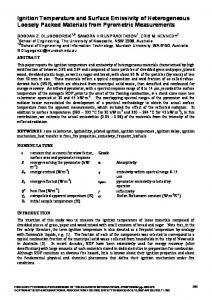
Fig. 1. Spectral variability of surface self-emission, atmospheric downward radiance, and ground-leaving radiance in 1132–1140 cm−1 , assuming a surface temperature at 300 K, a surface emissivity of 0.85, and a 1976 U.S. Standard Atmosphere.

where Latm↓,j is the equivalent atmospheric downward radiance ! 1 Latm↓,j = Latm↓,j (θi , φi ) cos θi dΩi . (3) π 2π

In a narrow spectral region of less than 15 cm−1 , the Planck function can be approximated as the linear function of the wavenumber. The surface emissivity changes slowly with the wavenumber and can be approximated as a constant. The first term of the right side of (2) is the surface self-emission that can be approximated as the linear function of the wavenumber in a narrow spectral region. The atmospheric downward spectral radiance contains sharp atmospheric emission lines and exhibits strong spectral contrasts. As shown in (2), since the groundleaving spectral radiance is equal to the surface self-emission plus the reflected atmospheric downward spectral radiance, it contains the reduced atmospheric emission at the positions of atmospheric emission lines and cannot be approximated as the linear function of the wavenumber in general. The relationship between the surface self-emission, atmospheric downward spectral radiance, and ground-leaving spectral radiance is shown in Fig. 1, where the surface temperature and emissivity are assigned to be 300 K and 0.85 at all wavenumbers, respectively, and the atmospheric downward spectral radiance is simulated by MODTRAN 4.0 with a 1976 US Standard Atmosphere [37]. The fact that the ground-leaving radiance spectrum cannot be approximated by a linear function of the wavenumber is caused primarily by the strong emission line of the atmospheric downward spectral radiance. The recovery of surface self-emission from (2) needs precise emissivity, assuming that ground-leaving radiance spectrum and the atmospheric downward spectral radiance are known; otherwise, the recovered surface self-emission radiance contains the residue of atmospheric downward spectral radiance. Given an initial emissivity estimate at the position of the strong emission line, if the emissivities are assumed to be

Authorized licensed use limited to: Rochester Institute of Technology. Downloaded on February 24,2010 at 08:44:40 EST from IEEE Xplore. Restrictions apply.

1590

IEEE TRANSACTIONS ON GEOSCIENCE AND REMOTE SENSING, VOL. 48, NO. 3, MARCH 2010

Fig. 2. Calculated surface self-emission with a series of given emissivities.

Fig. 4. Calculated distance BD corresponding to the data in Fig. 2. The minimum coincides with an emissivity of 0.85. TABLE I S IX NARROW S PECTRAL R EGIONS U SED TO D ERIVE S URFACE T EMPERATURE

surface temperature Ts from the radiometric measurements at the position of the atmospheric emission line as follows: " # Lks − (1 − εk )Latm↓,k −1 Ts = B (4) εk Fig. 3. One of the calculated surface self-emission cases with a given emissivity of 0.95.

constant in the narrow spectral region, we can calculate the surface self-emission radiance. If the given surface emissivity is equal to the true value of emissivity at the position of the atmospheric emission line, the calculated surface self-emission radiance does not contain the residue of the atmospheric downward spectral radiance, as shown in Fig. 2. Otherwise, the calculated surface self-emission radiance contains obvious atmospheric downward spectral radiance. The residue of atmospheric downward spectral radiance in the calculated selfemission radiance can be used to determine the suitability of the initial emissivity estimate. The degree of the residue of atmospheric downward spectral radiance can be characterized by distance BD in Fig. 3, where B is the point at the position of the atmospheric emission line, D is the point on line AC, and its abscissa is the same as point B. If the initial emissivity estimate is the most suitable, its corresponding residue will be the least. As we can see from Fig. 4, the distance is the least when its corresponding emissivity is 0.85. Since it is difficult to determine which initial emissivity estimate is more accurate than the others, we propose a stepwise refining method to determine the surface emissivity εk at the position of the atmospheric emission line and derive the

where B −1 represents the inverse function of the Planck function, and k is the position of the atmospheric emission line. To reduce the effect of instrumental random noise, we select six narrow spectral regions in 840–1220 cm−1 containing strong emission lines of water vapor to execute the algorithm (Table I). Temperature is derived at each selected spectral region. The final surface temperature Tˆ is determined as the mean of these six temperatures, and surface emissivity can be calculated as follows: εj =

Ljs − Latm↓,j . Bj (Tˆ) − Latm↓,j

(5)

In this algorithm, it is crucial to select a narrow spectral region that contains strong atmospheric emission lines. After the spectral regions are selected, the procedure of refining surface emissivity at the position of the atmospheric emission line can be described separately in four steps, as shown in Fig. 5. 1) Assign a series of inaccurate initial emissivity estimates with 0.1 interval at the position of the strong atmospheric emission line. Surface self-emission is calculated by assuming that the surface emissivity in the narrow spectral region is equal to the initial emissivity estimate. If one of the initial emissivity estimates matches the actual value, the calculated distance BD will be the least among all the calculated distances. In this step, we obtain an optimized

Authorized licensed use limited to: Rochester Institute of Technology. Downloaded on February 24,2010 at 08:44:40 EST from IEEE Xplore. Restrictions apply.

CHENG et al.: STEPWISE REFINING ALGORITHM OF TEMPERATURE AND EMISSIVITY SEPARATION

Fig. 5. Flow diagram of surface emissivity refinement at the position of the atmospheric emission line.

initial emissivity estimate (e-step1) at the position of the strong atmospheric emission line. 2) Generate a series of increasingly accurate initial emissivity estimates around e-step1 at 0.01 interval. After repeating step 1), we obtain a refined initial emissivity estimate (e-step2) at the position of the strong atmospheric emission line. 3) Repeat step 2) based on the refined initial emissivity estimate e-step2 with an emissivity interval of 0.001. A more accurate initial emissivity estimate (e-step3) is obtained from this step. 4) Repeat step 3) based on the refined initial emissivity estimate e-step3 at an emissivity interval of 0.0001. The final refined surface emissivity estimate (e-step4) at the position of the atmospheric emission line is obtained. III. N UMERICAL E XPERIMENTS The numerical experiments are first conducted to test the temperature and emissivity retrieval accuracy using our new algorithm. The results of TES from in situ measurements will be given in the next section. A. Data Preparation The simulated data set in the numerical experiments is composed of two parts: ground-leaving spectral radiance and atmospheric downward spectral radiance. A total of 1208 atmospheric profiles from the Thermodynamic Initial Guess Retrieval (TIGR) database with water content ranging from 0.40 to 7.36 g/cm2 are selected to model the atmospheric downward spectral radiance using MODTRAN4.0. For each atmospheric profile, ten surface temperatures are randomly generated using a Gaussian function with the mean value equal to the surface temperature of the profile and a standard deviation of 3 K; ten surface emissivity spectra are randomly chosen from 150 natural surface materials (Fig. 6) in the John Hopkins University (JHU) spectral library, including 96 rock samples, 41 soil samples, four vegetation samples, and nine samples

1591

Fig. 6. Subset of the selected emissivity spectra of various natural surface materials from the JHU spectral library.

of water, ice, and snow [38]. In the 714–1250 cm−1 spectral range, surface emissivities are interpolated into 2 cm−1 spectral intervals. The ground-leaving spectral radiance is calculated using (2). A random noise-equivalent spectral radiance (NESR) of 2.5 e−9 W/cm2 /sr/cm−1 , which is the labeled NESR of the ABB BOMEM MR 304 spectrometer, is added to the simulated 12 080 pairs of data. B. Results of Numerical Experiments The algorithm’s accuracy is characterized by two indices: temperature bias (Tbias ) and emissivity root-mean-square error (rmse) Tbias = |Tˆ − Ttrue |

(6)

where Ttrue is the true temperature, Tˆ is the inverted temperature, and abs represents the absolute value. This index is used to evaluate the algorithm’s temperature retrieval accuracy $ % N %' % (εi,inv − εtrue )2 & . (7) RMSE = i=1 N

Equation (7) is applied to each spectral band, where εi,inv is the inverted emissivity, εtrue is the true emissivity, and N is the total number of measurements in each band. There are many bands in the 714–1250 cm−1 thermal infrared spectral region, and the accuracy of surface emissivity retrieval is not the same in each one. Thus, this index is used to evaluate the algorithm’s emissivity retrieval accuracy in each band. Fig. 7 shows the scatter plot of true surface temperatures versus the inverted surface temperatures. High surface temperatures correspond to low Tbias and vice versa; Tbias is 0.04 ± 0.04 K. For each band, rmse is shown in Fig. 8. In the extremities of the 714–1250 cm−1 spectral region, rmse is relatively large due to the atmospheric emission line residual in the derived surface emissivity, which results from imperfect estimated surface temperature. Without considering the conditions mentioned earlier, the rmse of the retrieved emissivity is below 0.002.

Authorized licensed use limited to: Rochester Institute of Technology. Downloaded on February 24,2010 at 08:44:40 EST from IEEE Xplore. Restrictions apply.

1592

IEEE TRANSACTIONS ON GEOSCIENCE AND REMOTE SENSING, VOL. 48, NO. 3, MARCH 2010

Fig. 7. Scatter plot of true surface temperatures versus temperature bias. Asterisk corresponds to the temperature bias of SRTES, and circle symbol represents the temperature bias of ISSTES.

Fig. 8.

RMSE for each band.

TABLE II I NFLUENCE OF D IFFERENT L EVELS OF NESR AND S YSTEMATIC C ALIBRATION E RRORS ON S URFACE T EMPERATURE R ETRIEVAL

C. Comparison With the ISSTES Algorithm The ISSTES algorithm was originally proposed by Borel [27], for TES from hyperspectral thermal infrared data, and has proved to be an effective algorithm with high accuracy of temperature and emissivity retrieval [31], [36], [39]. In the ISSTES algorithm, surface emissivity is considered a smooth function of the wavenumber compared to the atmospheric downward spectral radiance which contains numerous gaseous emission lines. Emissivity spectra are first computed using a series of surface temperatures near the true surface temperature. Then, the smoothness of emissivity spectra is iteratively computed, and the smoothest emissivity spectrum is selected as the best estimation of surface emissivity. The corresponding temperature is regarded to be the best estimate of surface temperature. To demonstrate the advantages of our new algorithm, we use the ISSTES to derive surface temperature and emissivity with the same data used in Section III-A and compare the results with the stepwise refining temperature and emissivity separation (SRTES). As shown in Fig. 7, there exist some larger Tbias ’s which are introduced by the singular emissivities resulted from the instability of (5) in the point of numerical calculation. The value of Tbias is 0.14 ± 0.67 K. It should be pointed out that the true surface temperature lies within the 6-K range of given surface temperatures. Large Tbias definitely causes large rmse, as shown in Fig. 8. The rmse of the retrieved emissivity is below 0.012, excluding the extremities of the 714–1250 cm−1 spectral region. D. Sensitivity Analysis The required inputs of our algorithm are the ground-leaving radiance and atmospheric downward radiance, which are available after atmospheric correction. No atmospheric correction is perfect, and there are always errors associated with it. The errors related to these two quantities can propagate into the derived surface temperature and emissivity. The potential errors include random instrumental noise, instrument calibration error, and the atmospheric downward radiance error.

Fig. 9. RMSE for each band at different levels of NESR and systematic calibration errors.

Sensitivities to NESR and Systematic Calibration Errors: The influences of random instrumental noise on the accuracy of surface temperature and emissivity retrieval are investigated by adding different levels of noise equivalent spectral errors on the simulated ground-leaving spectral radiance and the atmospheric downward spectral radiance. The results are shown in Table II and Fig. 9. When the NESR is equal to the labeled NESR of the ABB BOMEM MR 304 spectrometer, i.e., 2.5 e−9 W/cm2 /sr/cm−1 , Tbias is 0.04 ± 0.04 K and increases to 0.36 ± 0.37 K as the NESR increases to 2.5 e−8 W/cm2 /sr/cm−1 ; the rmse of the retrieved emissivity is below 0.002 when the NESR is 2.5 e−9 W/cm2 /sr/cm−1 , and the rmse of the retrieved emissivity is below 0.018 as NESR is increased to 2.5 e−8 W/cm2 /sr/cm−1 .

Authorized licensed use limited to: Rochester Institute of Technology. Downloaded on February 24,2010 at 08:44:40 EST from IEEE Xplore. Restrictions apply.

CHENG et al.: STEPWISE REFINING ALGORITHM OF TEMPERATURE AND EMISSIVITY SEPARATION

Fig. 10. Influence of the atmospheric downward radiance errors on surface emissivity retrieval.

In order to evaluate the influence of systematic calibration error on surface temperature and emissivity retrieval, 0.5 and 1.0 K systematic calibration errors were added to the noised ground-leaving spectral radiance and the atmospheric downward spectral radiance, respectively. The added NESRs are 2.5 e−9 and 2.5 e−8 W/cm2 /sr/cm−1 , respectively. As we can see from Table II and Fig. 9, Tbias becomes larger with the increased systematic calibration errors, and the systematic calibration errors have almost no influence on surface emissivity retrieval. A systematic calibration error can be thought of as an additive error. Its effect on the numerator of (5) is eliminated by a subtraction operation, as is its effect on the denominator because the retrieved Tbias is almost on the same order of the systematic calibration error, as shown in Table II. Sensitivities to Atmospheric Downward Radiance Errors: To investigate the influence of the atmospheric downward radiance error on the accuracy of surface temperature and emissivity retrieval, the temperature and moisture profiles of the selected 1208 atmospheric profiles in the TIGR database are shifted by ±1 K and ±10%, respectively, to generate the simulated atmospheric downward spectral radiance. The added NESR is 2.5 e−9 W/cm2 /sr/cm−1 . When the temperature and moisture profiles are shifted by 1 K and 10%, Tbias is 0.21 ± 0.19 K, and Tbias is 0.22 ± 0.20 K when the temperature and moisture profiles are shifted by −1 K and −10%. As shown in Fig. 10, the rmse of the retrieved emissivity is less than 0.007 when the temperature and moisture profiles are shifted by 1 K and 10%, and it is less than 0.006 when the temperature and moisture profiles are shifted by −1 K and −10%. The rmse of the retrieved emissivity is less than 0.002 when only an NESR of 2.5 e−9 W/cm2 /sr/cm−1 is considered. Therefore, the atmospheric downward radiance error caused by the changes in temperature and moisture profiles has a strong effect on surface temperature and emissivity retrieval. IV. E VALUATION OF THE N EW A LGORITHM U SING I N SIT U M EASUREMENTS A field campaign was conducted in June 2004 on the Programme Inter-disciplinaire de Recherche sur la Radiométrie

1593

Fig. 11. Emissivity spectra of selected ten samples calculated from the laboratory-measured hemispherical–directional reflectance using Kirchhoff’s law.

Fig. 12. Example of the field-measured ground-leaving spectral radiance and atmospheric downward spectral radiance spectra for sample maroc.

en Environnement Extérieur experiment site of the Office National d’Etudeset de Recherches Aérospatiales center of Fauga-Mauzac [40]. The ABB BOMEM MR 254 spectrometer and LABSPHERE infragold plate were used to obtain the radiometric data of ten samples and the corresponding atmospheric information, from which the ground-leaving spectral radiance and the atmospheric downward spectral radiance were derived. During the measurement, the LABSPHERE infragold plate was placed at the location of the sample and observed from the vertical direction. These samples include soils, rocks, and manmade materials. The spectral resolution was 4 cm−1 (sampling rate is equal to 2 cm−1 ). For each sample, ten measurements were obtained: seven for daytime and three for nighttime. In addition, the hemispheric–directional reflectance of these samples was obtained using a BRUCKER-EQUINOX and an integrating sphere in the laboratory. Fig. 11 shows the emissivity spectra of the selected ten samples for this study. A pair of the fieldmeasured data for sample maroc is shown in Fig. 12. For each sample, the emissivity derived from laboratorymeasured hemispherical–directional reflectance using

Authorized licensed use limited to: Rochester Institute of Technology. Downloaded on February 24,2010 at 08:44:40 EST from IEEE Xplore. Restrictions apply.

1594

IEEE TRANSACTIONS ON GEOSCIENCE AND REMOTE SENSING, VOL. 48, NO. 3, MARCH 2010

Fig. 13. Emissivity rmse of each band for ten samples. The fine line represents the rmse of SRTES and the thick line for ISSTES rmses. The dotted line corresponds to an rmse of 0.01. (a) Ardoi. (b) Bois. (c) Maroc. (d) Negev. (e) Pie02. (f) Pie03. (g) Pie06. (h) Pstyr. (i) SablF. (j) Sic. Authorized licensed use limited to: Rochester Institute of Technology. Downloaded on February 24,2010 at 08:44:40 EST from IEEE Xplore. Restrictions apply.

CHENG et al.: STEPWISE REFINING ALGORITHM OF TEMPERATURE AND EMISSIVITY SEPARATION

Kirchhoff’s law is considered as the true value. Using the field measurements of atmospheric downward spectral radiance and ground-leaving spectral radiance, the SRTES and ISSTES algorithms are used to retrieve the emissivity spectra, and rmse is calculated for each band using the laboratorymeasured emissivities as truth. Fig. 13 shows the emissivity rmse of each band for ten samples. From Fig. 13, we can see the following: 1) On the whole, the rmse derived by the SRTES algorithm is about 0.01 except for sample pstyr; 2) the rmse is relatively large when sample emissivity is relatively low, which has also been found by Kaiser [41]; and 3) the rmse derived by the SRTES algorithm is lower than that derived by the ISSTES algorithm. Thus, we can conclude that the new algorithm is more accurate. V. D ISCUSSION In Section II, we presented a series of examples by assuming that surface emissivity was 0.85 at all wavenumbers in the narrow spectral region. Emissivities in the narrow spectral region are not equal. Equation (2) can be rearranged as follows by assuming a mean emissivity ε¯ in the narrow spectral region Ljs = (¯ ε + ∆εj )Bj (Ts ) + (1 − ε¯ − ∆εj )Latm↓,j

(8)

where ∆εj is the difference between ε¯ and εj . Surface selfemission radiance can be derived from (8), assuming that the surface emissivity at the position of the atmospheric emission lines is a constant c ( ) Lje = ε¯Bj (Ts ) + (c − ε¯)Latm↓,j + ∆εj Bj (Ts ) − Latm↓,j (9) where Lje represents the calculated self-emission radiance. In the narrow spectral region, ∆εj is on the order of about 0.001. Bj (Ts ) − Latm↓,j makes the last term on the right side of (9) even smaller, which can be neglected compared with the first two terms. Thus, the constant emissivity in the narrow spectral region is not a prerequisite, which has been validated in the TES using both numerically simulated data and in situ measurements. Assuming that (5) is used to calculate emissivity from hyperspectral data, the probability of introducing singular emissivity is very large when the difference between ground-leaving radiance and an object’s blackbody radiation at a given temperature is in the same order as the random instrumental noise [33], which implies that the probability of introducing singular emissivity is very large when the difference between the groundleaving radiance, the atmospheric downward radiance, and the object’s blackbody radiation at a given temperature is in the same order as the random instrumental noise. Singular emissivity imposes some constraints used in the previous algorithms, e.g., smooth assumption and correlation criterion will not be in effect. This, in turn, influences the surface temperature retrieval and produces larger Tbias at the end, as shown in Fig. 7. The SRTES algorithm is able to obtain an initial emissivity estimate under any circumstances, which may be inaccurate, but should not deviate too far from true emissivity if the algorithm’s assumption holds true. Moreover, six temperatures retrieved

1595

from the six narrow spectral regions are averaged as the final estimate of surface temperature, which will make Tbias even smaller. Thus, the SRTES algorithm can achieve high accuracy of surface temperature and emissivity retrieval, which can be seen from Figs. 7, 8, and 12. VI. C ONCLUSION In this paper, an SRTES algorithm has been proposed based on the analysis of the relationship between surface selfemission radiance and atmospheric downward radiance in a narrow spectral region. The SRTES algorithm utilizes the residue of atmospheric downward radiance in the calculated surface self-emission radiance as a criterion and adopts a stepwise refining method to determine the emissivity at the location of an atmospheric emission line in a narrow spectral region. Surface temperature is then determined. The mean value of six temperatures derived at six narrow spectral regions in 840–1220 cm−1 is considered to be the final estimate of surface temperature, which is then used to calculate surface emissivity. The numerical experiments are first used to investigate the accuracy of the algorithm and to carry out sensitivity analyses. A total of 1208 atmospheric profiles from the TIGR database, 150 natural surface materials from the JHU spectral library, and ten surface temperatures are combined together to generate the simulated data set. When an NESR of 2.5 e−9 W/cm2 /sr/cm−1 is added into the simulated data, Tbias is 0.04 ± 0.04 K, and the rmse of the retrieved emissivity is below 0.002 except in the extremities of the 714–1250 cm−1 spectral region. The results of the sensitivity analysis show that the systematic calibration errors of 0.5 and 1.0 K have significant influence on surface temperature retrieval and almost no influence on emissivity retrieval. The atmospheric downward radiance error and random instrumental noise have significant impacts on temperature and emissivity estimation, but the SRTES algorithm can still achieve high accuracy of temperature and emissivity retrievals. The SRTES algorithm is then applied to in situ measurements. The average emissivity rmse of ten samples is about 0.01 in the 750–1050 cm−1 spectral region and is 0.02 in the 1051–1250 cm−1 spectral region. Emissivity rmse is relatively large when sample emissivity is relatively low. The ISSTES algorithm is also used to retrieve surface temperature and emissivity from both simulated data sets and in situ measurements. The comparison analysis between the SRTES and ISSTES algorithms strongly suggests that the SRTES algorithm can overcome some common drawbacks in the existing physically based hyperspectral TES algorithms and achieve high accuracy of retrieved temperature and emissivity. At this time, we assume that the atmospheric effect of the remotely sensed data has been successfully corrected and the input of our algorithm is known. This is not always the case. In the future, we will extract atmospheric correction parameters and estimate the atmospheric downward spectral radiance from airborne/spaceborne thermal infrared hyperspectral data. The extension of the SRTES to other data sets of varying spectral regions and resolutions, from AQUA/AIRS’s nearly 0.5 cm−1 spectral resolution [42] to SEBASS’s 7 cm−1 spectral resolution at 890 cm−1 [14], is underway.

Authorized licensed use limited to: Rochester Institute of Technology. Downloaded on February 24,2010 at 08:44:40 EST from IEEE Xplore. Restrictions apply.

1596

IEEE TRANSACTIONS ON GEOSCIENCE AND REMOTE SENSING, VOL. 48, NO. 3, MARCH 2010

ACKNOWLEDGMENT The authors would like to thank the anonymous reviewers for their valuable comments and suggestions, Prof. Z. Li for providing the in situ measurements, and Dr. C. Russell for editing the manuscript. R EFERENCES [1] J. Sun and L. Mahrt, “Determination of surface fluxes from the surface radiative temperature,” J. Atmos. Sci., vol. 52, no. 8, pp. 1096–1106, Apr. 1995. [2] X. Li, A. Strahler, and M. Fridel, “A conceptual model for effective directional emissivity from nonisothermal surfaces,” IEEE Trans. Geosci. Remote Sens., vol. 37, no. 5, pp. 2508–2517, Sep. 1999. [3] F. Jacob, A. Olioso, X. Gu, Z. Su, and B. Seguin, “Mapping surface fluxes using visible, near infrared, thermal infrared remote sensing data with a spatialized surface energy balance model,” Agronomie, vol. 22, pp. 669–680, 2002. [4] L. Zhou, R. E. Dickinson, Y. Tian, M. Jin, K. Ogawa, H. Yu, and T. Schmugge, “A sensitivity study of climate and energy balance simulations with use of satellite-derived emissivity data over Northern Africa and the Arabian Peninsula,” J. Geophys. Res., vol. 108, no. D24, p. 4795, 2003, DOI: 10.1029/2003JD004083. [5] M. Jin and S. Liang, “An improved land surface emissivity parameter for land surface models using global remote sensing observations,” J. Clim., vol. 19, no. 12, pp. 2867–2881, Jun. 2006. [6] E. Péquignot, A. Chédin, and N. A. Scott, “Infrared continental surface emissivity spectra retrieved from AIRS hyperspectral sensor,” J. Appl. Meteorol. Clim., vol. 47, no. 6, pp. 1619–1633, Jun. 2008. [7] S. Liang, Quantitative Remote Sensing of Land Surfaces. Hoboken, NJ: Wiley, 2004. [8] R. D. Jackson, R. J. Reginato, and S. B. Idso, “Wheat canopy temperature: A practical tool for evaluating water requirements,” Water Resour. Res., vol. 13, no. 3, pp. 651–656, 1977. [9] F. N. Kogan, “Application of vegetation index and brightness for drought detection,” Adv. Space Res., vol. 15, no. 11, pp. 91–100, 1995. [10] T. R. McVicar and D. L. B. Jupp, “The current and potential operational uses of remote sensing to aid decisions on drought exception circumstances in Australia: A review,” Agric. Syst., vol. 57, no. 3, pp. 399–468, 1998. [11] Z. Wan, P. Wang, and X. Li, “Using MODIS land surface temperature and normalized difference vegetation index products for monitoring drought in the Southern Great Plains, USA,” Int. J. Remote Sens., vol. 25, no. 1, pp. 61–72, Jan. 2004. [12] A. B. Kahle, D. P. Madura, and J. M. Soha, “Middle infrared multispectral aircraft scanner data: Analysis for geological applications,” Appl. Opt., vol. 19, no. 14, pp. 2279–2290, Jul. 1980. [13] S. J. Hook, A. R. Gabell, A. A. Green, and P. S. Kealy, “A comparison of techniques for extracting emissivity information from thermal infrared data for geological studies,” Remote Sens. Environ., vol. 42, no. 2, pp. 123–135, Nov. 1992. [14] L. Kirkland, K. Herr, E. Keim, P. Adams, J. Salisbury, J. Hackwell, and A. Treiman, “First use of airborne thermal infrared hyperspectral scanner for compositional mapping,” Remote Sens. Environ., vol. 80, no. 3, pp. 447–459, Jun. 2002. [15] R. G. Vaughan, W. M. Calvin, and J. V. Taranik, “SEBASS hyperspectral thermal infrared data: Surface emissivity measurement and mineral mapping,” Remote Sens. Environ., vol. 85, no. 1, pp. 48–63, Apr. 2003. [16] L. C. Rowan, J. C. Mars, and C. J. Simpson, “Lithologic mapping of the Mordor, NT, Australia ultramafic complex by suing the Advanced Spaceborne Thermal Emission and Reflection Radiometer (ASTER),” Remote Sens. Environ., vol. 99, no. 1/2, pp. 105–126, Nov. 2005. [17] S. Liang, Ed., Advances in Land Remote Sensing: System, Modeling, Inversion and Application. New York: Springer-Verlag, 2008. [18] A. R. Gillespie, “Lithologic mapping of silicate rocks using TIMS,” in Proc. TIMS Data Users’ Workshop, 1985, pp. 29–44. [19] F. Becker and Z. Li, “Temperature-independent spectral indices in thermal infrared bands,” Remote Sens. Environ., vol. 32, no. 1, pp. 17–33, Apr. 1990. [20] K. Watson, “Two-temperature method for measuring emissivity,” Remote Sens. Environ., vol. 42, no. 2, pp. 117–121, Nov. 1992a. [21] Z. Li and F. Becker, “Feasibility of land surface temperature and emissivity determination from AVHRR data,” Remote Sens. Environ., vol. 43, no. 1, pp. 67–85, Jan. 1993.

[22] Z. Wan and Z. Li, “A physics-based algorithm for retrieving land surface emissivity and temperature from space,” IEEE Trans. Geosci. Remote Sens., vol. 35, no. 4, pp. 980–996, Jul. 1997. [23] K. Watson, “Spectral ration methods for measuring emissivity,” Remote Sens. Environ., vol. 42, no. 2, pp. 113–116, Nov. 1992. [24] P. S. Kealy and S. J. Hook, “Separating temperature and emissivity in thermal infrared multispectral scanner data: Implications for recovery of land surface temperatures,” IEEE Trans. Geosci. Remote Sens., vol. 31, no. 6, pp. 1155–1164, Nov. 1993. [25] A. Barducci and I. Pippi, “Temperature and emissivity retrieval from remotely sensed images using the grey body emissivity method,” IEEE Trans. Geosci. Remote Sens., vol. 34, no. 3, pp. 681–695, May 1996. [26] A. R. Gillespie, S. I. Rokugawa, T. Matsunaga, J. S. Cothern, S. Hook, and A. B. Kahle, “A temperature and emissivity separation algorithm for Advanced Spaceborne Thermal Emission and Reflection Radiometer (ASTER) images,” IEEE Trans. Geosci. Remote Sens., vol. 36, no. 4, pp. 1113–1126, Jul. 1998. [27] C. C. Borel, “Surface emissivity and temperature retrieval for a hyperspectral sensor,” in Proc. IEEE Int. Geosci. Remote Sens. Symp., T. I. Stein, Ed., 1998, vol. 1, pp. 546–549. [28] C. C. Borel, “Error analysis for a temperature and emissivity retrieval algorithm for hyperspectral imaging data,” Int. J. Remote Sens., vol. 29, no. 17/18, pp. 5029–5045, Sep. 2008. [29] Q. Liu and X. Xu, “The retrieval of land surface temperature and emissivity by remote sensing data: Theory and digital simulation,” J. Remote Sens., vol. 2, no. 1, pp. 1–9, 1998. [30] S. Liang, “An optimization algorithm for separating land surface temperature and emissivity from multispectral thermal infrared imagery,” IEEE Trans. Geosci. Remote Sens., vol. 39, no. 2, pp. 264–274, Feb. 2001. [31] R. O. Knuteson, F. A. Best, D. H. DeSlover, B. J. Osborne, H. E. Revercomb, and W. L. Smith, “Infrared land surface remote sensing using high spectral resolution aircraft observations,” Adv. Space Res., vol. 33, no. 7, pp. 1114–1119, 2004. [32] J. Cheng, Q. Xiao, X. Li, Q. Liu, and Y. Du, “Multi-layer perceptron neural network based algorithm for simultaneous retrieving temperature and emissivity from hyperspectral FTIR data,” Spectrosc. Spectr. Anal., vol. 28, no. 4, pp. 780–783, Apr. 2008. [33] J. Cheng, Q. Liu, X. Li, Q. Xiao, Q. Liu, and Y. Du, “Correlation-based temperature and emissivity separation algorithm,” Sci. China, ser. D, vol. 51, no. 3, pp. 357–369, Mar. 2008. [34] J. A. Sobrino, J. C. Jiménez-Muñoz, G. Sòria, M. Romaguera, L. Guanter, J. Moreno, A. Plaza, and P. Martinez, “Land surface emissivity retrieval from different VNIE and TIR sensors,” IEEE Trans. Geosci. Remote Sens., vol. 46, no. 2, pp. 316–327, Feb. 2008. [35] V. Payan and A. Royer, “Analysis of temperature and emissivity separation (TES) algorithm applicability and sensitivity,” Int. J. Remote Sens., vol. 25, no. 1, pp. 15–37, Jan. 2004. [36] P. M. Ingram and A. H. Muse, “Sensitivity of iterative spectrally smooth temperature/emissivity separation to algorithmic assumptions and measurement noise,” IEEE Trans. Geosci. Remote Sens., vol. 39, no. 10, pp. 2158–2167, Oct. 2001. [37] A. Berk, G. Anderson, P. Acharya, M. Hoke, J. Chetwynd, L. Bernstein, E. Shettle, M. Matthew, and S. Adler-Golder, MODTRAN4 Version 3 Revision 1 User’s Manual. Hanscom AFB, MA: Air Force Res. Lab., 2003. [38] J. W. Salisbury and D. M. D’Aria, “Emissivity of terrestrial materials in the 8–14 µm atmospheric window,” Remote Sens. Environ., vol. 42, no. 2, pp. 83–106, Nov. 1992. [39] J. Cheng, Q. Xiao, Q. Liu, and X. Li, “Effects of smoothness index on the accuracy of iterative spectrally smooth temperature/emissivity separation algorithm,” J. Atmos. Environ. Opt., vol. 2, pp. 376–380, 2007. [40] K. Kanani, L. Poutier, F. Nerry, and M. Stoll, “Directional effects consideration to improved Out-Door emissivity retrieval in the 3–13 µm domain,” Opt. Express, vol. 15, no. 19, pp. 12 464–12 482, Sep. 2007. [41] R. D. Kaiser, “Quantitative comparison of temperature/emissivity algorithm performance using SEBASS data,” Proc. SPIE, vol. 3717, pp. 47–57, Apr. 5–6, 1999. [42] M. T. Chahine, T. S. Pagano, H. H. Aumann, R. Atlas, C. Barnet, J. Blaisdell, L. Chen, M. Divakarla, E. J. Fetzer, M. Goldberg, C. Gautier, S. Granger, S. Hannon, F. W. Irion, R. Kakar, E. Kalnay, B. H. Lambrigtsen, S.-Y. Lee, J. Le Marshall, W. W. McMillan, L. McMillin, E. T. Olsen, H. Revercomb, P. Rosenkranz, W. L. Smith, D. Staelin, L. L. Strow, J. Susskind, D. Tobin, W. Wolf, and L. Zhou, “The Atmospheric Infrared Sounder (AIRS): Improving weather forecasting and providing new insights into climate,” Bull. Amer. Meteorol. Soc., vol. 87, no. 7, pp. 911–926, Jul. 2006, DOI: 10.1175/BAMS-87-7-911.

Authorized licensed use limited to: Rochester Institute of Technology. Downloaded on February 24,2010 at 08:44:40 EST from IEEE Xplore. Restrictions apply.

CHENG et al.: STEPWISE REFINING ALGORITHM OF TEMPERATURE AND EMISSIVITY SEPARATION

Jie Cheng received the B.Sc. degree in survey and mapping from the East China Institute of Technology, Fuzhou, China, in 2002 and the Ph.D. degree in cartography and remote sensing from the Institute of Remote Sensing Applications, Chinese Academy of Sciences, Beijing, China, in 2008. He is currently undertaking postdoctoral research with the State Key Laboratory of Remote Sensing Science, Beijing Normal University/Chinese Academy of Sciences, Beijing, and the Research Center for Remote Sensing and GIS, Beijing Normal University, Beijing. His main research interests focus on surface temperature and emissivity retrieval from hyperspectral data, surface emissivity modeling, and trace gas inversion using remotely sensed data. Shunlin Liang (M’94–SM’01) received the Ph.D. degree in remote sensing and geographic information systems from Boston University, Boston, MA. He was a Postdoctoral Research Associate with Boston University from 1992 to 1993 and a Validation Scientist with the National Oceanic Atmospheric Administration (NOAA)/National Aeronautics and Space Administration (NASA) Pathfinder Advanced Very High Resolution Radiometer Land Project from 1993 to 1994. He is currently a Professor with the University of Maryland, College Park. He authored the book Quantitative Remote Sensing of Land Surfaces (Wiley, 2004) and edited the book Advances in Land Remote Sensing: System, Modeling, Inversion and Application (Springer, 2008). His main research interests focus on spatiotemporal analysis of remotely sensed data, integration of data from different sources and numerical models, and linkage of remote sensing with global environmental changes. He is a member of NASA Advanced Spaceborne Thermal Emission and Reflection Radiometer and Moderate-Resolution Imaging Spectroradiometer science teams and the NOAA Geostationary Operational Environmental Satellite-R Series Land science team. Dr. Liang is the Cochairman of the International Society for Photogrammetry and Remote Sensing Commission VII/I Working Group on Fundamental Physics and Modeling. He is an Associate Editor of the IEEE T RANSACTIONS ON G EOSCIENCE AND R EMOTE S ENSING and also a Guest Editor of several remote sensing journals.

1597

Jindi Wang received the B.S. degree from the Beijing University of Posts and Telecommunications, Beijing, China, in 1982. She is currently a Professor with the State Key Laboratory of Remote Sensing Science, Beijing Normal University/Chinese Academy of Sciences, Beijing, and the Research Center for Remote Sensing and GIS, Beijing Normal University, Beijing. Her primary research interests focus on land surface bidirectional reflectance distribution function modeling, land surface parameter retrieval from various remotely sensed data, and typical land surface objects’ spectrum library building and its applications.

Xiaowen Li received the B.S. degree from Chengdu Institute of Radio Engineering, Chengdu, China, in 1968 and the M.A. degree in geography in 1981, the M.S. degree in electric and computer engineering in 1985, and the Ph.D. degree in geography from the University of California, Santa Barbara. He is currently with the State Key Laboratory of Remote Sensing Science, Beijing Normal University/Chinese Academy of Sciences, Beijing, China; the Research Center for Remote Sensing and GIS, Beijing Normal University, Beijing; and the Institute of Remote Sensing Applications, Chinese Academy of Sciences, Beijing. Before this, he was a Research Professor with the Center for Remote Sensing, Department of Geography, Boston University, Boston, MA. He established the vegetation bidirectional reflection Li-Strahler geometric optics model. He initiated the ill-conditioned inversion theory in the field of quantitative remote sensing. On the study of the applicability of the Helmholtz reciprocity principle in the area of ground surface remote sensing, he put forward the limitation conditions of Helmholtz reciprocity principle for the nonuniform image element bidirectional reflection. With respect to the scale effect of Planck’s law in ground surface remote sensing, he set up the conceptual model suitable for nonisothermal surface heat-radiation direction and initiated the scale modifier formula of Planck’s law for nonisothermal blackbody plane.

Authorized licensed use limited to: Rochester Institute of Technology. Downloaded on February 24,2010 at 08:44:40 EST from IEEE Xplore. Restrictions apply.