A Stochastic Model for Interconnection Complexity based ... - CiteSeerX

A Stochastic Model for Interconnection Complexity based on Rent’s Rule Peter Verplaetse∗ Dirk Stroobandt† Jan Van Campenhout Department of Electronics and Information Systems Ghent University, Belgium {pvrplaet|dstr|jvc}@elis.rug.ac.be

Abstract In the past, Rent’s rule has been successfully applied for a priori estimation of wire length distributions. Deviations to Rent’s rule appear due to the existence of heterogeneity. This can be classified in hierarchical and spatial heterogeneity. Stochastic models for the interconnection complexity, based on Rent’s rule, are introduced. A coarse model shows that the variance follows a power law relationship. A more refined model incorporates the effect of local spatial heterogeneity. Experiments show that this is sufficient to model the variance of the terminal count distribution. Finally, the model is further extended to incorporate global spatial heterogeneity.

1

Introduction

The interconnection complexity of a circuit is well captured by Rent’s rule [1] and the corresponding Rent exponent. This rule has been applied numerous times, especially in the field of a priori wire length estimation [2, 3, 4]. Because of the absence of placement and routing information, it is impossible to accurately estimate the length of individual nets, but the wire length distribution can be predicted fairly accurately. Larger Rent exponents result in more flat wire length distributions, with relatively more long wires. This results in a larger average wire length and hence a larger total wiring area. Since the wiring area dominates the total area of contemporary chips, it seems valuable to include the Rent exponent in the cost objective during synthesis. Measurement of the Rent exponent seems fairly expensive, as it requires partitioning the circuit into smaller modules. But when using a divide-by-conquer approach for synthesis, the partitioning and thus the Rent exponent can be obtained “for free”.

Furthermore, a priori wire length estimation could be extremely valuable for the interaction between logic synthesis and physical design. During synthesis, tight wire length constraints can be set on the individual nets, which allows accurate delay estimation. Because of the accurate estimation of the wire length distribution, the wire length constraints can be met during the physical design stage. This approach could guarantee timing closure without requiring many design iterations. Nevertheless many researchers remain suspicious about the use of Rent’s rule: it is an empirical law that holds on average, but there are many cases where significant deviations exist. These deviations result mainly from heterogeneity in the circuit. Circuit heterogeneity comes in two forms: hierarchical heterogeneity and spatial heterogeneity. The former is well known and has been studied thoroughly [1, 3, 5, 6, 7]. The latter has had little attention so far – yet it is known to have a huge impact on the accuracy of wire length estimations based on Rent’s rule [5]. Spatial heterogeneity results in spread on the Rent characteristic. As shown in [8], the amount of variance is a fundamental property of circuits, and has a direct influence on the difficulty of finding good partitionings of the circuit. In this paper we will study the deviations from Rent’s rule. After an overview of the basic definitions and Rent’s rule in the next section, we will briefly discuss hierarchical heterogeneity. In section 4 we will focus on the spatial heterogeneity. First, a coarse model that takes the logic block degree distribution into account will be derived. This model will be refined to incorporate the effect of local spatial heterogeneity. Finally the model will be further extended to model global spatial heterogeneity as well.

2

Preliminaries

∗

Research Assistant of the Fund for Scientific Research – Flanders (Belgium)(F.W.O.) † Post-doctoral Fellow of the Fund for Scientific Research – Flanders (Belgium)(F.W.O.)

In this section we will give an overview of the basic definitions and we continue with a discussion on Rent’s rule.

Logic block Net Terminal Module

(a)

(b)

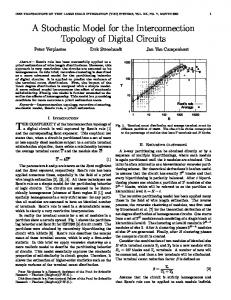
Figure 1: Model of a circuit (a) and the partitioning of the circuit into modules (b).

2.1

Definitions

A circuit can be represented by a set of interconnected blocks, as in figure 1(a) (the blocks can be the representation of transistors, gates or even entire circuits). An interconnection between two or more blocks is called a net. A net that is connected to more than two blocks is called a multi-terminal net. Some of the nets are also connected to the outside world. These nets are called external nets, as opposed to the internal nets which only connect blocks within the circuit. In order to model these external nets properly, we introduce a new kind of block which we call a terminal. The other blocks are called logic blocks. Every external net is connected to exactly one terminal. The circuit size is defined as the number of logic blocks contained by the circuit. The terminal count T corresponds to the number of terminals of the circuit. The logic block degree t is the number of nets incident to the logic block. The logic block degree distribution Dt is the collection of values, indicating for each t, how many logic blocks have a logic block degree equaling t. Partitioning a circuit means dividing this circuit into disjoint sub-circuits (called modules), each containing a subset of the blocks (figure 1(b)). Generally the criterion for partitioning is to minimize the number of nets cut, i.e. the number of nets crossing the borders of modules in the partition. Recently, it has been observed that minimizing the number of terminals is a better criterion than minimizing the number of nets cut and that both criteria are not equal for multi-terminal external nets [9]. Nets that are cut by module boundaries are shared between two or more modules and are said to be external to the modules. Therefore, the net is split into a number of sub-nets (if the net was already external to the circuit then the terminal assigned to it can be reused for one of the sub-nets). Each module itself can be seen as a circuit and can be partitioned further. A partitioning process where the modules themselves are recursively

partitioned is called a hierarchical partitioning method. For a partition P, the terminal count distribution DT (P) is a collection of values, indicating for each terminal count T , how many modules have exactly T terminals. One usually considers partitions of more or less equally sized modules. These partitions are identified by the average module size B, and the corresponding terminal count distribution is written as DT (B). At the lowest level of a hierarchical partitioning of a circuit, where every module contains a single logic block, the terminal count distribution equals the logic block degree distribution, hence DT (1) = Dt .

2.2

Rent’s rule

Circuits can be classified according to their interconnection structure. These differences in complexity of the interconnection topology have been experimentally observed by Rent, and his observations have led to the wellknown Rent’s rule [1]. This law states that, when partitioning a circuit in a number of more or less equally sized modules, there exists a power law relationship between the average terminal count T and the average number of logic blocks B: T = kB

p

(1)

Here, k corresponds to the average logic block degree t, and p is the Rent exponent. The validity of this rule is a result of the self-similarity [11] that exists in real circuits. A high Rent exponent implies many global interconnections, and hence a high interconnection complexity. Generally, p ranges from 0.47 for regular circuits, such as Random Access Memories, up to 0.75 for complex circuits, such as fast full custom VLSI circuits [12]. The visualization of the terminal count distribution as function of the module size is called the Rent characteristic, as shown in figure 2).

100 – 70 – 50 – 33 – 25 – 18 – 13 – % 10 – 7– 5–

100

T 10

3– 2–

1

1–

1

10

B

100

1000

Figure 2: Rent characteristic of LGsynth93 [10] circuit apex5. The size of the circles corresponds to the percentage of modules that has T terminals and B blocks in a pool of modules around an average number of blocks. Since partitioning algorithms are heuristic, the solution is not guaranteed to be optimal. As a result, the terminal count distribution and the resulting Rent exponent is not only determined by the circuit itself, but also depends on the partitioning algorithm [13]. The results obtained from these suboptimal partitions are still relevant, since similar partitioning schemes are used in contemporary placement tools. For the experimental results reported in this paper, we have used a recursive partitioning scheme, where at each hierarchical level the modules are bipartitioned using hMetis [14].

3

Hierarchical heterogeneity

While recursively partitioning a circuit, the observed Rent exponent may vary across the different levels of hierarchy. The deviation at the highest levels of hierarchy results in Rent region II [1], as opposed to region I, which is the region where (1) is valid. The deviation at the lowest levels results in Rent region III [6]. This piecewise linear approximation1 of Rent’s rule models the hierarchical heterogeneity quite well, as shown in figure 3. Region II At the highest levels of the hierarchy the number of terminals quite often appear to be lower than expected by (1). This behavior can be intrinsic to the functionality of the circuit, but is mostly due to technological and psychological constraints [7]. The most important technological constraint is the pinlimitation of contemporary packages. As a result, various coding techniques, such as time multiplexing and compression, are used in order to maximize the entropy that is transported across the circuit pins. A similar technological constraint exists for circuit submodules, 1 In

the log-log domain.

Region III

Region I

Region II

100

T

10

1

1

10

100

B

1000

Figure 3: Rent characteristic for circuit s9234.1. since these are interconnected through busses, and the number of bus lines should be minimized to minimize the total number of global wires. Quite often, designers are too much aware of these constraints. They are indoctrinated to use as little terminals as possible, which results in a psychological constraint.

Region III During the logic synthesis phase the circuit is mapped to a certain technology. The logic block degree distribution seems more or less independent from the circuit and is mainly determined by the logic blocks that are available in the technology. As a result, the average logic block degree, and thus the average terminal count for modules of size B = 1 (lowest level of the hierarchy) is mostly determined by the technology and mainly independent from the circuit and its complexity. When a mismatch exists between the average logic block degree and the k parameter in (1), which corresponds to Rent region I, a region III is observed. The factor k is meaningless for the actual circuit com-

plexity. Consider the case where the logic blocks are simple logic gates, without macro cells such as IP cores. A typical average logic block degree would be t = 3.5. Now look at the internals of the logic gates, which actually consist of transistors. Changing the viewpoint does not alter the circuit complexity, even though the average logic block degree is different. The Rent characteristic appears to be shifted to higher module sizes, but the Rent characteristic and the corresponding Rent exponent does not change significantly in Region I and II. Because of the smaller granularity, we expect the partitioning tool to find finer cuts, but apparently this only has influence on the lower levels of the hierarchy.

a certain amount of spread at the other levels of the hierarchy (B > 1). This can be demonstrated with the following stochastic model. Consider the opposite of recursive partitioning the circuit: the bottom-up clustering of the logic blocks into modules, and further combining those modules to a complete circuit. First consider the combination of two modules of identical size B and terminal count T into a new module with Bc = 2B blocks and Tc terminals. Because of the self-similarity, the number of terminals that is reduced is determined by Rent’s rule: Tc = kBcp = k(2B)p = 2p T

(2)

A similar effect appears when the circuit is mapped to The total terminal count before combination was 2T , different technologies: the Rent characteristics and cor- therefore in a single combination step the number of terresponding Rent exponents (at least in Regions I and minals is reduced by a factor α: Tc II) seem independent of the technology the circuit is = 2p−1 (3) α= mapped to during logic synthesis [15]. 2T Of course, because of the logic block degree distribution, the modules that are combined will not be identical. However, since the circuits are partitioned with a con4 Spatial heterogeneity straint on the maximum imbalance, the number of blocks will be similar. Experiments show that the allowed maxFor a priori wire length estimation, a simplified circuit imum imbalance does not fundamentally change the termodel based on Rent’s rule is frequently used. In this minal count distribution.3 model one assumes that the terminal count for each module complies exactly to Rent’s rule, i.e. the termi- For modules with different terminal count, the fraction nal count distributions are assumed to be concentrated α is assumed to be independent of the true number of at a single value given by Rent’s rule.2 In reality these terminals, such that the number of terminals of a module distributions exhibit a certain spread, which is partly the at hierarchical level k, where B = 2k , is given by: result of the logic block degree distribution, but mainly (4) T(2k ) = αk (t1 + t2 + · · · + t2k ) determined by deviations from Rent’s rule (spatial heterogeneity). Visually, when inspecting the Rent char- In this expression ti are random variables with distribuacteristics, the amount of spread seems to diminish for tion defined by the logic block degree distribution. Since increasing block size, due to the compressing effect of every bipartitioning in the recursive partitioning scheme the logarithmic scale. In reality the amount of spread, is performed locally, i.e. without considering the cost which can be characterized by the variance of the termi- functions of the bipartitionings at the same and lower nal count distribution, increases for increasing module levels of the hierarchy, the ti variables in the reverse clustering scheme can be assumed to be mutually insize. dependent. The expected value and the variance of the In this section we will model the influence of the logic terminal count distribution at hierarchical level k is then: block degree distribution. Then we will refine this model (5) E[T(2k )] = αk 2k E[t] = 2kp E[t] by adding spatial heterogeneity. We will focus mainly on k 2k k (2p−1)k Var[t] (6) Var[T(2 )] = α 2 Var[t] = 2 the variance of the terminal count distribution, but we will briefly inspect the shape of the distributions as well. Since the logic block degree distribution is fixed, the ex-

4.1

pected value and variance can easily be measured as the mean t and sample variance σt2 of this distribution. SubInfluence of the logic block degree stituting for the module size B we get:

distribution

E[T(B)] = B p t

(7)

For B = 1, i.e. the lowest level of hierarchy in a re(8) Var[T(B)] = B (2p−1) σt2 cursive partitioning scheme, the spread of the terminal The first expression reduces to Rent’s rule with k = t. count distribution is determined by the logic block de- When the Rent exponent p > 0.5, the variance increases. gree distribution. Because of this distribution, we expect 2 Rounded

to the nearest integer.

3 At least not when using an advanced partitioning algorithm such as hMetis.


k 2Var[α]E[T(1)]2  For p = 0.5, the variance remains constant, and for 4E[α]2 + 2 E[α] − Var[α] p < 0.5 it decreases. Figure 4 shows actual and predicted
k  variance for ISPD98 circuit ibm02, which has a Rent ex− 2E[α]2 + 2Var[α] ponent of 0.705. The existence of a power law relation 
k ship is confirmed, but the measured exponent does not 2σα2 2 2α2 + 2σα2 E[t] = Var[t] − 2 comply with (7). Of course the measurement of the Rent α − σα2 exponent is not exact, but in this case a Rent exponent 2σ 2 +4 2 α 2 E[t]2 α2k (13) of 1.114 would be required to obtain a fairly good match. α − σα This is nonsense, since a Rent exponent can never exceed 1. This indicates that the influence of the logic block deAfter substituting for the module size B = 2k this results gree distribution is only minor, and that the model needs in: further refinement. (14) E[T(B)] = B p t   10000 2 2 2σ 2 2 Var[T(B)] = σt2 − 2 α 2 t B 1+log2 (α +σα ) α − σα 1000 2 2σ 2 + 2 α 2 t B 2p (15) α − σ 2 α σT 100 Expression (14) is again Rent’s rule. The variance consists of two terms. Since α ∈ [0, 1] and for p > 0.4, 10 α > 0.66, the variance σα2 will always be significantly Measured variance Modeled variance (p=0.705) smaller than α2 . Therefore the exponent of the first Modeled variance (p=1.114) term will be approximately 2p − 1, such that the second 1 term will dominate for sufficiently large module size. 1 10 100 1000 B

Figure 5 shows the variance for circuit ibm01. The rent exponent of 0.588 results in a fairly good fit for the variFigure 4: Measured and predicted variance for circuit ance, but a much better fit can be obtained with rent ibm02 (modeled without local heterogeneity). exponent of 0.805. This is probably due to global heterogeneity, which will be discussed further.

4.2

10000

Local spatial heterogeneity

In the previous model, we considered the factor α to be constant. In reality, this factor will also be a random variable, with mean α = 2p−1 and variance σα2 determined by the amount of local variety in the selfsimilarity. As a result, the variance of the terminal count distribution will increase much faster.
(9) T(2k ) = α T1 (2k−1 ) + T2 (2k−1 ) k−1

1000

σT

2

100

10

Measured variance Modeled variance (p=0.588) Modeled variance (p=0.805)

k−1

) and T2 (2 ) to be stochastically Assume α, T1 (2 independent. The expected value and the variance of the terminal count distribution becomes: E[T(2k )] = 2E[α]E[T(2k−1 )]

(10)

Var[T(2k )] = 2Var[α]Var[T(2k−1 )] +4Var[α]E[T(2k−1 )]2 +2Var[T(2k−1 )]E[α]2 Solving these recursive relationships yields: E[T(2k )] = 2k E[α]k E[T(1)] = 2kp E[t]
k Var[T(2k )] = Var[T(1)] 2E[α]2 + 2Var[α]

(11)

1

1

10

100

1000

B

Figure 5: Measured and predicted variance for circuit ibm01 (modeled with local heterogeneity). The parameter σα2 was obtained by optimizing for best fit.

In table 1 the results for all ISPD98 circuits are showed. For each circuit expression (15) is fitted twice: in the first (12) case the Rent exponent p is fixed to the measured value, and only the variance σα2 is optimized; in the second case both p and σα2 are optimized. In both cases the average

Circuit ibm01 ibm02 ibm03 ibm04 ibm05 ibm06 ibm07 ibm08 ibm09 ibm10 ibm11 ibm12 ibm13 ibm14 ibm15 ibm16 ibm17 ibm18

p 0.588 0.705 0.659 0.676 0.715 0.632 0.645 0.632 0.604 0.631 0.629 0.654 0.630 0.628 0.630 0.620 0.661 0.612

Fixed p 2 σα 0.036 0.038 0.067 0.086 0.045 0.040 0.070 0.111 0.062 0.063 0.056 0.102 0.066 0.076 0.085 0.075 0.060 0.104

Error 0.0133 0.0031 0.0097 0.0625 0.0190 0.0047 0.0044 0.0706 0.0080 0.0219 0.0108 0.0356 0.0109 0.0360 0.0088 0.0070 0.0021 0.0240

p 0.805 0.662 0.581 0.364 0.621 0.650 0.669 0.399 0.569 0.540 0.582 0.531 0.566 0.504 0.588 0.577 0.659 0.707

Optimized 2 σα 0.006 0.052 0.114 0.382 0.091 0.034 0.058 0.390 0.083 0.133 0.084 0.243 0.111 0.195 0.122 0.107 0.061 0.050

p Error 0.0018 0.0011 0.0042 0.0057 0.0040 0.0040 0.0036 0.0042 0.0061 0.0025 0.0075 0.0066 0.0037 0.0022 0.0036 0.0023 0.0021 0.0031

datapath and memory), or by the synthesis tool (example: a fast multiplier that consists of a Wallace tree of carry-save adders and a fast carry-lookahead adder). When hierarchically partitioning a global heterogeneous circuit, the heterogeneity will become apparent at the highest levels of the hierarchy: the circuit falls apart into smaller sub-circuits that are globally homogeneous. This can easily be incorporated into the stochastic model, since the global heterogeneity determines a partitioning of the logic blocks into distinct classes. When clustering the different logic blocks and resulting modules, only those logic blocks and modules that consist of the same class can be combined.

The resulting terminal count distributions are a mixture of distributions that correspond to global homogeneous Table 1: Variance fit for ISPD98 benchmark circuits. circuits. Consider a global heterogeneous circuit that consists of n sub-circuits of size B1 , B2 , ..., Bn , with logarithmic error is minimized. Except for a few circuits, corresponding terminal count distributions DT1 , DT2 , ..., such as ibm04 and ibm08, the model allows a good fit, DTn . The terminal count is then given by: especially when the Rent exponent is adjusted as well. (16) T(B) = Tj (B)

4.3

Global spatial heterogeneity

So far we only analyzed the variance of the terminal count distributions. For some applications the actual shape of the distributions could be important. In the previously derived model, the terminal count at each hierarchical level is a sum of random variables. Because of the shared α factors, these random variables are not mutually independent. Hence, the central limit theorem does not apply, and the shape of the terminal count distributions will depend on the distribution of α. We inspected the normalized terminal count distribution for a variety of logic block degree distributions and α distributions. According to our model, the terminal count distribution converges quickly to a distribution that seems bell-shaped, but is skewed towards smaller terminal counts. The terminal count distributions of most large ISPD98 circuits seem to have a similar shape. This shape is shown in figure 6(b). Note that it is actually quite hard to measure the terminal count distribution of real circuits, since the number of sample points decreases exponentially due to the recursive partitioning scheme.

where j is a discrete random variable with distribution defined by the size of the sub-circuits: Bj (17) Dj = B1 + B2 + · · · + Bn The calculation of the expected value and variance is straightforward: n X Di E[Ti (B)] (18) E[T(B)] = i=1

Var[T(B)] =

n X

Di E[Ti (B)2 ] − E[T(B)]2

i=1

=

n X

Di Var[Ti (B)] + E[Ti (B)]2




i=1

−E[T(B)]2

(19)

From the last expression it is clear that the variance consists of multiple terms. When substituting (14) and (15) for E[Ti (B)] and Var[Ti (B)], we get a sum of exponential terms. Thus global heterogeneity adds degrees of freedom to the stochastic modal, but does not fundamentally change the nature of the expression for the variance. The extra degrees of freedom will obviously result in a better fit, but the gain seems only marginal, since a fairly good fit was already obtained with the preSome of the smaller ISPD98 circuits converge to a vious model. platykurtic distribution, i.e. a flat topped distribution, or even a multimodal distribution, as shown in figure 6(a) for circuit ibm01. This indicates that the circuits are Conclusion actually a mixture of different sub-circuits, each with 5 different Rent exponent. This global spatial heterogeneity exists in many circuits. It is either introduced by the Deviations to Rent’s rule appear due to the existence of designer (example: a circuit that consists of a controller, heterogeneity. Hierarchical heterogeneity can be mod-

0.5

0.5

0.4

pT

0.4

0.3

pT

0.2 0.1

0.3 0.2 0.1

0

0 1

1

B

16

8 32 -2

-1

0

1

B

2

512

σ

-2

(a) ibm01

-1

0

1

2

σ

(b) ibm18

Figure 6: Normalized terminal count distribution for circuits ibm01 and ibm18. eled by splitting up Rent’s rule in different regions according to the module size, which results in a piecewise linear approximation of Rent’s rule. The terminal count distribution exhibits a certain amount of spread, which is partly the result of the logic block degree distribution, but mainly due to spatial heterogeneity. A coarse model for the terminal count distribution has been derived to take the logic block degree distribution into account. This model was further refined to account for the local spatial heterogeneity. The result is a simple yet accurate model that is sufficient to describe the variance of the terminal count distribution quite accurately. Further extensions are possible to incorporate the effects of global spatial heterogeneity. This results in a more complex model that is capable of describing both the variance and the shape of the terminal count distribution.

[6]

[7]

[8]

[9]

[10]

References [1] B. S. Landman and R. L. Russo. On a pin versus block relationship for partitions of logic graphs. IEEE Trans. on Comput., vol. C–20: pages 1469–1479, 1971. [2] W. E. Donath. Wire length distribution for placements of computer logic. IBM J. of Research and Development, vol. 25: pages 152–155, 1981. [3] D. Stroobandt. Analytical methods for a priori wire length estimates in computer systems, November 1998. Ph.D. thesis (translated from Dutch), University of Ghent, Faculty of Applied Sciences. [4] J. A. Davis, V. K. De, and J. D. Meindl. A stochastic wire-length distribution for gigascale integration (GSI) – PART I: Derivation and validation. IEEE Trans. on Electron Devices, vol. 45 (no. 3): pages 580–589, March 1998. [5] H. Van Marck, D. Stroobandt, and J. Van Campenhout. Towards an extension of Rent’s rule for describing local variations in interconnection complexity. In S. Bai,

[11]

[12]

[13]

[14]

[15]

J. Fan, and X. Li, editors, Proc. 4th Intl. Conf. for Young Computer Scientists, pages 136–141. Peking University Press, 1995. D. Stroobandt. On an efficient method for estimating the interconnection complexity of designs and on the existence of region III in Rent’s rule. In M. A. Bayoumi and G. Jullien, editors, Proc. 9th Great Lakes Symposium on VLSI, pages 330–331. IEEE Computer Society Press, March 1999. H. Van Marck. Kwantitatieve studie en modellering van opto-elektronische driedimensionale interconnectiestructuren, March 2000. Ph.D. thesis (in Dutch), University of Ghent, Faculty of Applied Sciences. D. Stroobandt, P. Verplaetse, and J. Van Campenhout. Generating synthetic benchmark circuits for evaluating CAD tools. Technical Report PARIS 00-01, University of Ghent, Belgium, ELIS Department, January 2000. D. Stroobandt. Pin count prediction in ratio cut partitioning for VLSI and ULSI. In M. A. Bayoumi, editor, Proc. IEEE Intl. Symp. on Circuits and Systems, pages VI–262–VI–265. IEEE, May 1999. Computer-Aided Design Benchmarking Laboratory. Available at: http://www.cbl.ncsu.edu/benchmarks/. P. Christie. A fractal analysis of interconnection complexity. Proc. of the IEEE, vol. 81 (no. 10): pages 1492– 1499, 1993. R. L. Russo. On the tradeoff between logic performance and circuit-to-pin ratio for LSI. IEEE Trans. Comput., vol. C–21: pages 147–153, 1972. L. Hagen, A. B. Kahng, F. J. Kurdahi, and C. Ramachandran. On the intrinsic Rent parameter and spectra-based partitioning methodologies. IEEE Trans. on Comput.-Aided Des., Integrated Circuits & Syst., vol. 13 (no. 1): pages 27–37, January 1994. G. Karypis and V. Kumar. hMetis: A Hypergraph Partitioning Package, November 1998. Available at: http://www-users.cs.umn.edu/~karypis/metis/ hmetis/main.shtml. P. Verplaetse. On the relationship between rent’s rule and pareto points. Technical Report PARIS 00-04, University of Ghent, Belgium, ELIS Department, April 2000.