A Stochastic Programming Model for the Thermal Optimal Day-Ahead Bid Problem with Physical Futures Contracts Cristina Corchero and F.-Javier Heredia Dept. of Statistics and Operations Research Universitat Polit`ecnica de Catalunya, Barcelona (Spain)
DR 2009/03 16 February 2009
Copies of this report may be downloaded at http://hdl.handle.net/2117/2795
Corresponding author:
F. Javier Heredia Dept. Statistics and Operations Research, Technical University of Catalonia, Campus Nord c. Jordi Girona 1-3, 08034 Barcelona, tel. (0034) 934017335 fax. (0034) 934015855 email:
[email protected]
A Stochastic Programming Model for the Thermal Optimal Day-Ahead Bid Problem with Physical Futures ContractsI Cristina Corcheroa , F.-Javier Herediaa,∗ a Department
of Statistics and Operations Research, Universitat Politecnica Catalunya. Barcelona, Spain.
Abstract The reorganization of the electricity industry in Spain completed a new step with the start-up of the Derivatives Market. One main characteristic of MIBEL’s Derivatives Market is the existence of physical futures contracts; they imply the obligation to settle physically the energy. The market regulation establishes the mechanism for including those physical futures in the day-ahead bidding of the Generation Companies. The goal of this work is to optimize coordination between physical futures contracts and the Day-Ahead bidding which follow this regulation. We propose a stochastic quadratic mixed-integer programming model which maximizes the expected profits, taking into account futures contracts settlement. The model gives the simultaneous optimization for the Day-Ahead Market bidding strategy and power planning production (unit commitment) for the thermal units of a price-taker Generation Company. The uncertainty of the day-ahead market price is included in the stochastic model through a set of scenarios. Implementation details and some first computational experiences for small real cases are presented. Key words: Stochastic programming, OR in energy, electricity day-ahead market, futures contracts, optimal bid 1. Introduction In recent there has been a reorganization of the electricity industry. The deregulation of the generation and distribution of electricity carried out in most countries in Europe has changed the problems that the generation companies (GenCo) have to face. With the introduction of the Electricity Markets, the price of electricity has become a significant risk factor. One of the techniques for hedging against market-price risk is participation in futures markets (Deng and Oren, 2006) and, for this reason, the creation of Derivatives Electricity Markets has been a natural step in the deregulation process. I The
work of C. Corchero was supported by FPI Grant BES-2006-12311,
On the Spanish mainland, the Electricity Market, which was launched in 1998, includes a Day-Ahead Market, a Reserve Market and a set of balancing and adjustment markets. As the introduction of competition and the deregulation process did not behave as expected, the Spanish market was improved in 2007 with the start-up of the Iberian Electricity Market (MIBEL) and some other new regulations. The MIBEL brings together the Spanish and Portuguese electricity systems and it complements the previous Spanish Electricity Market with a Derivatives Market. Generation companies can no longer optimize their short-term generation planning decisions without considering the relationship between those markets. Among the products that the Derivatives Market offers, we
and the work of F.-Javier Heredia was partially supported by Grants DPI2005-
will focus on the futures contracts. In the MIBEL Derivatives
09117-C02-01 and DPI2008-02153, all of them grants of the Ministry of Sci-
Market, an average 2340GWh are traded monthly (Fig. 1). A
ence and Innovation of Spain ∗ Corresponding author. Address: Ed. C5-206, Campus Nord, Jordi Girona
futures contract is an exchange-traded derivative that represents
1-3 08034 Barcelona. Spain. Tel.: +34-934-017-335. Fax: +34-934-015-855 Email addresses:
[email protected] (Cristina Corchero),
agreements to buy/sell some underlying asset in the future at a specified price (Hull, 2002). The main characteristics of a fu-
[email protected] (F.-Javier Heredia) Preprint submitted to Elsevier
March 18, 2009
the optimal bid curves of a hydro-thermal system. Nowak et al.
3000 Month Quarter Year
(2005) and Fleten and Kristoffersen (2007) also distinguish be-
2500
tween the variables representing the bid energy and those corGWh
2000
responding to the matched energy in the case of a price-taker GenCo. In particular, Fleten and Kristoffersen (2007) has some
1500
aspects that are very related to this work; it presents a stochas-
1000
tic programming model to optimize the unit commitment and
500
the day-ahead bidding of a hydropower producer in the Nord 0 jun − 07
jul − 07
aug − 07
sept − 07
oct − 07 nov − 07 Month
dec − 07
jan − 08
feb − 08
mar − 08
Pool. Finally, Heredia et al. (2008a) and Heredia et al. (2008b), propose an optimal bid function similar to the one introduced
Figure 1: MIBEL Futures contracts traded energy
in this work where, instead of futures contracts, there are bilateral contracts to be satisfied. Moreover, general considerations
tures contract are the asset; the contract size; the delivery ar-
about optimal bidding construction in electricity markets can
rangements and period; and the characteristics of the price. In
be obtained in Anderson and Philpott (2002) and Anderson and
contrast to other Electricity Derivatives Markets, the delivery
Xu (2002). Neither of these studies mentioned includes futures
arrangements of the MIBEL futures contract offer a choice be-
contracts.
tween a physical or financial settlement. Physical futures con-
Some different approaches to the inclusion of futures con-
tracts have cash settlement and physical delivery whereas finan-
tracts in the management of a GenCo can be found in the elec-
cial contracts have cash settlement only. This physical delivery
tricity market literature. Most of the literature defines forward
option is the feature of the futures contract that interacts with
contracts as contracts with a physical settlement and futures
the GenCo day-ahead bidding process (OMEL, 2007).
contracts as contracts with a financial settlement. The main
In liberalized electricity markets, a GenCo must build an
theoretical differences between these two kinds of derivatives
hourly bid that is sent to the market operator, who selects the
products is the level of standardization and the kind of market
lowest price among the bidding companies in order to match the
where they are traded (Hull, 2002). We focus on the inclusion of
pool load. Some earlier studies give the optimal bidding quan-
physical derivatives products in the short-term management of
tity once the expected distribution of the spot prices is known
a GenCo, other general considerations about futures contracts
(Shrestha et al., 2004; Triki et al., 2005) but do not propose any
can be found in many works, for instance, Hull (2002), Collins
explicit modelization of the optimal bid. Conejo et al. (2002)
(2002), Neuberger (1999) or Carlton (1984).
proposes an optimal stepwise bidding strategy for a price-taker
Prior to deregulation, Kaye et al. (1990) illustrates how phys-
GenCo based on the units characteristics, the expected spot
ical and financial contracts can be used to hedge against the
price, and the optimal generation. Furthermore, Gountis and
risk of profit volatility, allowing for flexible responses to spot
Bakirtzis (2004) considers the approximation of stepwise bid
price. After day-ahead and derivatives markets start-up, Bjor-
curves by linear bid functions based on the marginal costs and
gan et al. (1999) presents a theoretical framework for the in-
the optimal generation quantity. Nabona and Pages (2007) gives
tegration of futures contracts into the risk management of a
a three stage procedure to build the optimal bid based on the op-
GenCo. Also, Chen et al. (2004) presents a bidding decision
timal generation quantity and the zero-price bid. Also, Ni et al.
making system for a GenCo taking into account the impacts
(2004) uses the concept of price-power function, which is sim-
of several types of physical and financial contracts; this sys-
ilar to the matched energy function used in our work, to derive
tem is based on a market-oriented unit commitment model, a 2
probabilistic local marginal price simulator, and a multi-criteria
is developed and its properties are described. In section 4, a
decision system. Furthermore, Conejo et al. (2008) optimizes
detailed case study is solved and analyzed. Finally, in section
the forward physical contracts portfolio up to one year, taking
5, some relevant conclusions are presented.
into account the day-ahead bidding; the objective of the study is 2. Model
to protect against the pool price volatility through futures contracts. Moreover, Guan et al. (2008) optimizes in a medium-
2.1. Coordination between Day-Ahead and Derivatives Mar-
term horizon the generation asset allocation between different
kets
derivatives products and the spot market, taking into account
As stated above, the MIBEL regulation (OMEL, 2007) de-
short-term operating constraints; it considers the known price
scribes the coordination between the physical futures contracts
of the contracts and forecasts the spot price. From another point
portfolio and the Day-Ahead bidding mechanism (Fig. 2). This
of view, Tanlapco et al. (2002) does a statistical study of the re-
coordination is structured in the following three phases:
duction in risk due to forward contracts; it is shown that, for a GenCo, the electricity futures contracts are better to hedge
1. For every derivatives contract in which the GenCo is inter-
price risk than other related futures as crude oil or gas futures
ested, it has to define the Term Contract Units (UCP in the
contracts.
MIBEL’s notation) which are virtual units allowed to be
As stated above, we are dealing with a new electricity fu-
offered in the Derivatives Market. Each UCP is formed by
tures contract situation due to the MIBEL definition of physical
the subset of the physical units of the GenCo which will
futures contracts, hence, as far as we know, there is no previous
generate the energy to cover the corresponding contract.
work dealing with the short-term management of the GenCo
For each contract, a physical unit can only participate in
which includes the coordination between day-ahead bidding strate-
one virtual UCP.
gies and physical futures settlement. The MIBEL regulation
2. Two days before the delivery date the GenCo receives from
(OMEL, 2007) describes the coordination between this physical
the Derivatives Market Operator, OMIP (OMIP, 2008) the
futures contracts portfolio and the Day-Ahead bidding mecha-
quantity that every UCP has to produce in order to cover
nism of the GenCo. That regulation obliges the GenCo to deter-
the matched futures contracts. This information is also
mine its generation scheduling in order to be able to cover those
sent to the Day-Ahead Market Operator, OMEL (OMEL,
obligations and to determine its optimal offer, taking into ac-
2008).
count those futures contracts. Following the idea that the partic-
3. OMEL demands that every GenCo commit the quantity
ipation in the Spot and the Derivatives Markets has to be studied
designated to futures contracts through the Day-Ahead Mar-
jointly, the main objective of this work is to build a stochastic
ket bidding of the physical units that form each UCP. This
programming model which includes the coordination between
commitment is made by the so called instrumental price
physical futures contracts and Day-Ahead Market bidding fol-
offer, that is, a sale offer with a bid price of 0e/MWh (also
lowing the MIBEL rules. In other words, we want to see how
called price acceptant).
the inclusion of futures contracts in the model affects the short
That regulation implies that the GenCo has to determine its
term strategies of the GenCo in the Day-Ahead Market.
unit commitment in order to be able to cover those obligations
In section 2, the stochastic programming model for the co-
and it has to determine its optimal bid by taking into account
ordination between day-ahead bidding and the physical futures
those instrumental price offers. Due to the algorithm the mar-
contract portfolio -taking into account thermal unit operational
ket operator uses to clear the Day-Ahead Market, all instrumen-
constraints- is presented. In section 3, the optimal bid function
tal price offers will be matched (i.e. accepted) in the clearing 3
2.2. First stage binary variables and thermal units operation constraints
UCP contract j j ∈F
Day-ahead market D ,s
λi
Thermal units
psit
uit t∈Tj
t∈T
The formulation of the start-up and shut-down processes qit t∈Tj
follows Nabona and Pages (2007). Let uit ∈ {0, 1} be a first-
Futures contracts
stage binary variable expressing the off-on operating status of the t th unit over the ith interval (uit = 1 if committed, uit = 0
Lj , λj j ∈F
if uncommitted). The values of uit and u(i+1)t must obey certain operating rules ini order to take into account the constraints
GenCo
of the minimum in service and idle time. It is necessary to introduce two extra binary variables eit and ait for each uit . Let
Figure 2: Representation of the system under study at period i
eit ∈ {0, 1} be a start-up indicator for the t th unit. It has a value of one in all intervals i where the t th unit has changed from
process, that is, this energy shall be produced and will be remu-
u(i−1)t = 0 to uit = 1, and zero elsewhere. Similarly, ait ∈ {0, 1}
nerated at the spot price.
is a shut-down indicator for the t th unit. It should have a value
Following MIBEL’s rules, if we are optimizing today we
of one in all intervals i where u(i−1)t = 1 to uit = 0, and zero
focus on tomorrow’s Day-Ahead Market because we have to
otherwise. The following three sets of constraints unambigu-
submit tomorrow’s bidding. Thus, the optimization horizon is at 24-hour intervals; this set of intervals is denoted as I. The
ously model the commitment variable uit and the star-up and
proposed short-term bidding strategies are addressed to a price-
shut-down variables eit and ait :
taker GenCo. The generation units to be considered are the thermal units with participation in the auction process. The rel-
uit + u(i−1)t − eit + ait = 0
evant parameters of a thermal unit are:
∑
akt ≤ 1
∀i ∈ I, ∀t ∈ T
(2)
ekt ≤ 1
∀i ∈ I, ∀t ∈ T
(3)
k=i
• quadratic generation costs with constant, linear and quadratic
of f
min{i+tt
coefficients, ctb (e), ctl (e/MWh) and ctq (e/MWh) respectively, for the
(1)
min{i+tton ,|I|}
eit +
t th
∀i ∈ I, ∀t ∈ T
ait +
,|I|}
∑
k=i+1
unit.
2.3. First stage continuous variables and futures contracts cov-
• Pt and Pt the upper and lower bound, respectively, on the
ering constraints
energy generation (MWh) of a committed unit t.
Let qit be the first-stage variable standing for the energy of • start-up, cton , and shut-down, cto f f , costs (e) for the t th
the instrumental price offer, that is, the energy bid by unit t to
unit. e
the ith day-ahead market at 0e/MWh. If variable fit j represents the energy of the jth futures contract allocated to thermal unit t
• minimum operation and minimum idle time, minton and
at period i, then the following constraints must be satisfied:
minto f f respectively, for the t th unit., i.e., the minimum number of hours that the unit must remain in operation
∑
fit j = L j
∀i ∈ I, ∀ j ∈ F
(4)
∀i ∈
(5)
t∈T j
once it is started up and the minimum number of hours
qit ≥
that the unit must remain idle once it has been shut down
∑
fit j
∀t ∈ T
∀ j∈Ft
before being started up again, respectively.
t
Pt uit ≤ qit ≤ P uit fit j ≥ 0 4
∀i ∈ I
∀t ∈ T
(6)
∀i ∈ I, ∀t ∈ T, ∀ j ∈ F
(7)
where the known parameters Ft , T j and L j are, respectively, the
Definition 2 (Matched energy function). The matched energy
subset of contracts in which unit t participates, the set of ther-
associated to the bid function λitb is defined as the maximum bid
mal units that participates in contract j (the units in all the UCPs
energy with an asked price not greater than the clearing price
that participate in the contract j) and the energy that has to be
λid , and is represented by the function:
settled for contract j. Constraint (4) ensures that the energy of the
jth
def
d b b b d pm it (λi ) = max{pit ∈ [0, Pt ] | λit (pit ) ≤ λi }
futures contracts L j will be completely dispatched
(9)
among all the committed units of its associated UCPs. Con-
The clearing price λid is a random variable that will be mod-
straints (5) formulate the MIBEL’s rule that forces the energy
eled through a set of scenarios S with associated spot prices
of the future contracts to be bid through the instrumental price
λ d,s = {λ1d,s , . . . , λId,s } and probabilities Ps = P(λ d,s ), s ∈ S.
offer. The lower bound qit ≥ Pt uit prevents committed ther-
Each one of these scenarios has, for each period i, a correspond-
mal units from being matched below their minimum generation
ing matched energy that will be represented in the model by
limit.
the second stage variable psit . Although our model will be developed without any assumption on the specific expression of
2.4. Second stage variables: matched energy
the bid function λitb it is necessary, for the sake of the model’s
The formulation of the objective function of the present
consistency, to assume the existence of a bid function with a
model will include variables representing the value of the matched matched energy function (9) that agrees with the optimal value
energy for the committed thermal unit t on the ith day-ahead
of variables psit , i.e.:
market. For the moment, the matched energy will be loosely
Assumption 1. For any thermal unit t committed at period i
defined as the accepted energy in the clearing process; that is,
there exists a bid function λitb such that:
the energy that the thermal t should generate at period i and that
d,s s∗ pm it (λi ) = pit
will be rewarded at the clearing price. This matched energy, which plays a central role in our model, is uniquely determined
∀s ∈ S
(10)
s with ps∗ it the optimal value of variable pit
by the sale bid and the clearing price. A sale bid in the MIBEL’s Notice that the existence of such a bid function is not evident, as
day-ahead market consists of a stepwise non-decreasing curve
all scenarios must prove simultaneously equal (10). The proof
defined by up to 10 energy (MWh)-price(e/MWh) blocks. As
of existence and the analytical expression of a bid function λitb
usual in this kind of work (see Gountis and Bakirtzis (2004))
satisfying (10) (optimal bid) will be developed in section 3.
we will consider a simplified modelization of the true sale bid
The matched energy psit is related to the rest of the first stage
through the so called bid function λitb , not necessarily stepwise:
variable through the following set of constraints:
Definition 1 (Bid function). A bid function for the thermal unit
psit ≤ Pt uit
∀i ∈ I, ∀t ∈ T, ∀s ∈ S
(11)
that gives, for any feasible value of the bid energy pbit , the asked
psit ≥ qit
∀i ∈ I, ∀t ∈ T, ∀s ∈ S
(12)
price per MWh from the day-ahead market:
qit ≥ Pt uit
∀i ∈ I, ∀t ∈ T
(13)
t is a non-decreasing function defined over the interval [0, Pt ]
λitb :
[0, Pt ] −→ ℜ+ ∪ 0 pbit
7−→ λitb (pbit )
This set of constraints substitutes the bounds on qit defined in
(8)
(6).
For a given bid function λitb the matched energy associated to the clearing price λid ,
pm it
2.5. Objective function
is defined through the matched energy
The expected value of the benefit function B can be ex-
function
pressed as: 5
h i Eλ d B(u, a, e, p; λid ) = ³ ´ ∑ ∑ λ jf − λid L j ∀i∈I ∀ j∈F
h i cton eit + ctof f ait
−∑
∑
+∑
∑ ∑ Ps
∀i∈I ∀t∈T
∀i∈I ∀t∈T ∀s∈S
(DABFC) : minimize ∑
(14)
p,q, f ,a,e,u
∑
³ cton eit + cto f f ait + ctb uit
∀i∈I ∀t∈T
h i´ + ∑ Ps (ctl − λid,s )psit + ctq (ptis )2
(15)
(17)
s∈S
h λid,s psit
s.t.
³ ´i − ctb uit + ctl psit +ctq (psit )2 (16)
∑
fit j = L j
∀i ∈ I, ∀ j ∈ F
(18)
∀i ∈ I, ∀t ∈ T
(19)
∀i ∈ I, ∀t ∈ T
(20)
∀i ∈ I, ∀t ∈ T
(21)
∀i ∈ I, ∀t ∈ T
(22)
psit ≤ Pt uit
∀i ∈ I, ∀t ∈ T, ∀s ∈ S
(23)
psit ≥ qit
∀i ∈ I, ∀t ∈ T, ∀s ∈ S
(24)
mal units. This term is deterministic and does not depend
qit ≥ Pt uit
∀i ∈ I, ∀t ∈ T
(25)
on the realization of the random variable λid .
fit j ≥ 0
∀i ∈ I, ∀t ∈ T, ∀ j ∈ F
(26)
uit , ait , eit ∈ {0, 1}
∀i ∈ I, ∀t ∈ T
(27)
t∈U j
qit ≥
where:
∑
fit j
j∈Ft
(14) is a constant term, which would be excluded from the op-
uit + u(i−1)t − eit + ait = 0 min{i+tton ,|I|}
timization, and corresponds to the incomes of the futures
∑
eit +
contracts. Futures contracts are settled by differences,
akt ≤ 1
k=i of f
i.e., each futures contract has daily cash settlement of the
min{i+tt
ait +
price differences between the market reference price λid
∑
,|I|}
ekt ≤ 1
k=i+1
and the futures settlement price λ jf . (15) is the on/off fixed cost of the unit commitment of the ther-
(16) represents the expected value of the benefit from the dayahead market, where Ps is the probability of scenario s.
In the next sections the properties of the optimal solutions
The first term, λid,s psit , computes the incomes from the
of the (DABFC) problem will be studied.
day-ahead market due to a value psit of the matched energy, while the term between parentheses corresponds
3. Optimal Bid
to the expression of the quadratic generation costs. Of course, ctb uit could have been added to the deterministic
The preceding model (17)-(27) is built on the assumption
term (15), as it doesn’t depend on the scenario, but it has
1, which presumes the existence of a bid function λitb with a
been conserved in (16) for the sake of clarity.
matched energy function consistent with the optimal solution of the (DABFC) problem, i.e.:
All the functions appearing in Eqs. (15) and (16) are linear except the term (16), which is concave quadratic (ctq ≥ 0, see
d,s s∗ pm it (λi ) = pit
∀s ∈ S
(28)
Table 4.1). The objective of this section is the development of such a bid function, called the optimal bid function λitb∗ (pbit ). In order
2.6. The Day-Ahead Bid with Futures Contracts problem The full model developed in the preceding sections, the so-
to derive this optimal bid function, the properties of the opti-
called Day-Ahead Bid with Futures Contracts problem can be
mal solutions of the problem (17)-(27) will be studied in the
formulated as:
next section and used to derive the expression of the optimal ∗ matched energy ps∗ it in terms of the instrumental energy bid qit .
6
3.1. Optimal matched energy Let x∗ 0 = [u∗ , a∗ , e∗ , p∗ , q∗ , f ∗ ]0 represent the optimal solu-
(DABFC∗i ) :
tion of the (DABFC) problem. Fixing the binary variables to its
∑∗ ∑ Ps
minimize
optimal value u∗ , a∗ and e∗ in the formulation of the (DABFC)
pi ,qi , fi
problem, we obtain the following convex quadratic continuous
∀t∈Toni s∈S
i h (ctl − λid,s )psit + ctq (psit )2
(36)
s.t.
problem:
∑
∀j ∈ F
(πi j )
(37)
∗ ∀t ∈ Ton i
(µ˜ it )
(38)
psit − Pt ≤ 0
∗ ∀t ∈ Ton , ∀s ∈ S i
(µ sit )
(39)
qit − psit ≤ 0
∗ ∀t ∈ Ton , ∀s ∈ S i
(µˆ its )
(40)
Pt − qit ≤ 0
∗ ∀t ∈ Ton i
(µ it )
(41)
− fit j ≤ 0
∗ ∀t ∈ Ton , ∀j ∈ F i
(µ˘ it j )
(42)
fit j − L j = 0
∗ t|t∈T j ∩Ton i
∑
(DABFC∗ ) : minimize ∑ p,q, f
∑
i h q s 2 d,s s s l P − λ )p + c (p ) (29) (c ∑ t t it it i
∗ s∈S ∀i∈I ∀t∈Ton i
s.t.
∑
fit j = L j
∀i ∈ I, ∀ j ∈ F
(30)
∗ t|t∈T j ∩Ton i
qit ≥
∑
fit j
∀i ∈ I, ∀t
j∈Ft
∗ ∈ Ton i
(31)
psit ≤ Pt
∗ , ∀s ∈ S ∀i ∈ I, ∀t ∈ Ton i
(32)
psit ≥ qit
∗ , ∀s ∈ S ∀i ∈ I, ∀t ∈ Ton i
(33)
qit ≥ Pt
∗ ∀i ∈ I, ∀t ∈ Ton i
(34)
fit j ≥ 0
∗ ∀i ∈ I, ∀t ∈ Ton , ∀j ∈ F i
(35)
fit j − qit ≤ 0
j∈Ft
where π , µ˜ , µ , µˆ , µ and µ˘ represent the Lagrange multiplier associated with each constraint. The Karush-Kuhn-Tucker conditions of the (DABFC∗i ) problem can be expressed as:
Ps
∗ := {t ∈ T | u∗ = 1}. Obviously, the optimal solution of with Ton it i
h³ ´ i ctl − λid,s + 2ctq ps∗ it + +µ sit − µˆ its = 0
this continuous problem should coincide with the optimal value
−µ˜ it − µ it +
of the continuous variables of the original (DABFC) problem, p∗ , q∗ and f ∗ . The (DABFC∗ ) problem is separable by inter-
∑ µˆ its = 0
∀s∈S
µ˜ it + πi j − µ˘ it j = 0 à !
vals, being the problem associated with the ith time interval in
µ˜ it
standard form (Luenberger (2004)):
∑
j∈Ft
fit j − q∗it
=0
∗ ∀t ∈ Ton , ∀s ∈ S i
(43)
∗ ∀t ∈ Ton i
(44)
∗ ∀t ∈ Ton , ∀ j ∈ Ft i
(45)
∗ ∀t ∈ Ton i
(46)
¡ ¢ ∗ µ sit ps∗ it − Pt = 0 ∀t ∈ Toni , ∀s ∈ S ∗ µ it (Pt − q∗it ) = 0 ∀t ∈ Ton i
(47) (48)
∗ µˆ its (q∗it − ps∗ it ) = 0 ∀t ∈ Toni , ∀s ∈ S
(49)
∗ µ˘ it j fit∗ j = 0 ∀t ∈ Ton , ∀j ∈ F i
(50)
∗ , ∀ j ∈ F, ∀s ∈ S (51) µ˜ it , µ sit , µ it , µˆ its , µ˘ it j ≥ 0 ∀t ∈ Ton i
The (DABFC∗i ) problem is convex (ctq ≥ 0) and then the system (43)-(51) represents the necessary and sufficient optimality conditions of the (DABFC∗i ) problem and, consequently, of the (DABFC∗ ) problem. Therefore the solution set of the preceding KKT system defines the value of variables psit , qit 7
(a) Pt < q∗it = ps∗ it = Pt : This is a trivial case, because, by def-
and fit j over the optimal solution of the (DABFC) problem as-
d,s s∗ ∗ inition (53), pd,s it ≤ Pt , and then pit = max{qit = Pt , pit ≤
∗ . The following lemma states this result: sociated with Ton i
Pt } = Pt .
Lemma 1. Let x∗ 0 = [u∗ , a∗ , e∗ , p∗ , q∗ , f ∗ ]0 be an optimal solu-
ˆ its = 0 that, to(b) Pt ≤ q∗it < ps∗ it = Pt : Condition (49) gives µ
tion of the (DABFC) problem. Then, for any x∗ there exists
gether with the non-negativity of the lagrange multipliers
Lagrange multipliers, µ˜ , µ , µˆ , µ and µ˘ such that the value
µ sit and equation (55) sets Pt ≤ θits and, by definition (53),
of variables p∗ , q∗ and f ∗ satisfy the KKT system (43)-(51). Conversely, for any solution (43)-(51) associated with
p∗ ,
∗ Ton i
q∗
and
f∗
d,s s∗ ∗ pd,s it = Pt . Then pit = max{qit < Pt , pit = Pt } = Pt
of the KKT system
(c) Pt ≤ q∗it < ps∗ it < Pt : In this case, conditions (47) and (49)
the correspondent solution x∗ is
give µ sit = µˆ its = 0, that, together with equation (55) gives
optimal for the (DABFC) problem.
d,s s s ∗ ps∗ it = θit < Pt . Then, by definition (53), pit = θit > qit d,s ∗ d,s s ∗ and ps∗ it = max{qit , pit = θit > qit } = pit
The fact that any solution of the (DABFC) problem must satisfy the system (43)-(51) will be exploited in the next two lemmas to
(d) Pt < q∗it = ps∗ it < Pt : In this case, condition (47) forces
derive the expressions of the optimal matched energy associated
µ sit = 0 which, in combination with equation (55) and con-
to scenario s:
∗ s dition µˆ its ≥ 0 gives ps∗ it = qit ≥ θit . Definition (53) sets a
Lemma 2 (Optimal matched energy, quadratic costs).
s value of pd,s it that will be either θit or Pt being in both cases
Let x∗
∗ d,s ∗ ∗ less than q∗it , and then ps∗ it = max{qit , pit ≤ qit } = qit
be an optimal solution of the (DABFC) problem. Then, for any unit t with quadratic convex generation cost (i.e. mitted at period i (i.e. t energy
ps∗ it
ctq
s (e) Pt = q∗it = ps∗ it < Pt : Condition (47) sets µ it = 0 which,
> 0) com-
by taking into account equation (55) and µˆ its ≥ 0, provides
∗ ), the optimal value of the matched ∈ Ton i
d,s s ps∗ it = Pt ≥ θit . Then, by definition (53), pit = Pt , and
can be expressed as:
d,s ∗ ps∗ it = max{qit = Pt , pit = Pt } = Pt
∗ d,s ps∗ it = max{qit , pit }
(52)
Before developing an analogous lemma for those thermal units with linear generation costs, it is necessary to introduce
where pd,s it is the constant parameter Pt s pd,s it = θit P t with
the following assumption:
if θits ≤ Pt
Assumption 2. For every t ∈ T with ctq = 0, λid,s 6= ctl ∀i ∈ I
if Pt ≤ θits ≤ Pt
(53)
and s ∈ S.
if θits ≥ Pt
³
¤
This assumption is not a severe restriction to our model, as for real instances of the problem it can always be accomplished
´
θits = λid,s − ctl /2ctq
by perturbing, if necessary, the price λid,s , with a small amount
(54)
ε ≈ 0 without any practical consequence. Proof As lemma 1 establishes, any optimal solution of the (DABFC) problem must satisfy the KKT system (43)-(51). As ctq > 0,
an optimal solution of the (DABFC) problem. If assumption 2
equation (43) allows variable ps∗ it to be expressed as: ps∗ it =
λid,s − ctl 2ctq
+
µˆ its − µ sit 2ctq Ps
= θits +
µˆ its − µ sit 2ctq Ps
Lemma 3 (Optimal matched energy, linear costs). Let x∗ be holds, then for any unit t with linear generation cost (i.e. ctq = ∗ ), the optimal value of the 0) committed at period i (i.e. t ∈ Ton i
(55)
matched energy ps∗ it can be expressed as: q∗ if λ d,s < ctl it i s∗ pit = Pt if λ d,s > cl t i
To derive the relationships (52), the solution of the KKT system will be analyzed in the following five cases, among which any optimal solution of the (DABFC) problem could be classified: 8
(56)
Proof As lemma 1 sets forth, any optimal solution of the (DABFC) problem and solution x∗ if the value of the matched energy funcproblem must satisfy the KKT system (43)-(51). When ctq = 0
d,s tion associated to any scenario’s clearing price λid,s , pm it (λi ),
equation (43) can be expressed as:
coincides with the optimal matched energy ps∗ it given by expres-
³ ´ µˆ its − µ sit = Ps ctl − λid,s
sions (52) and (56).
(57)
d,s s∗ The equivalence pm it (λi ) ≡ pit assures us that, if a GenCo
with Ps the probability of scenario s. There are two possible
submits systematically optimal bid functions to the day-ahead
cases:
market, the expected value of the benefits will be maximized,
(a) λid,s < ctl : in this case equation (57) impllies that µˆ its > µ sit
as long as the actual behaviour of the clearing price λid has
which gives rise to two different situations. In the first one
been captured by the set of scenarios S. The next lemma de-
µˆ its > µ sit > 0, that, together with equations (47) and (49)
velops the expression of the optimal bid function associated to
gives
ps∗ it
=
q∗it
= Pt . In the second one
the same KKT conditions forces
ps∗ it
=
µˆ its
q∗it
>
µ sit
= 0 and
the (DABFC) problem:
≤ Pt Lemma 4 (Optimal bid function). Let x∗ 0 = [u∗ , a∗ , e∗ , p∗ , q∗ , f ∗ ]0
(b) λid,s > ctl : now equation (57) sets µ sit > µˆ its , which again
be an optimal solution of the (DABFC) problem and t any ther-
defines only two possibilities. In the first one the strict
mal unit committed on period i at the optimal solution (i.e.
inequalities of µ sit > µˆ its > 0 hold and, considering equa-
∗ ). Then: t ∈ Ton i
∗ tions (47) and (49), set ps∗ it = qit = Pt . In the second one,
µ sit > µˆ its = 0 which, after equations (47) and (49), allows the matched energy to be expressed as
ps∗ it
= Pt ≥ q∗it .
(i) If the generation cost is quadratic convex, the bid function: 0 if pbit ≤ q∗it λitbq∗ (pbit ) = (58) 2cq pb + cl if q∗ < pb ≤ Pt t it t it it
¤
Lemmas 2 and 3 establish the expressions of the optimal matched energy variable for any spot price λid,s at any optimal solution of the (DABFC) problem. The bid strategies consis-
is optimal w.r.t. the (DABFC) problem and the optimum
tent with such a matched energy will be developed in the next
x∗ . (ii) If the generation cost is linear and assumption 1 holds, the
section.
bid function: 3.2. Optimal bid function In section 2.4 the concepts of bid and matched energy func-
λitbl∗ (pbit ) =
tions were introduced. The matched energy function associated with a given bid function λitb was defined as
0
if pbit ≤ q∗it
cl t
if q∗it < pbit ≤ Pt
(59)
is optimal w.r.t. the (DABFC) problem and the optimum x∗ .
def
d b b b d pm it (λi ) = max{pit ∈ [0, Pt ] | λit (pit ) ≤ λi }
Proof We will consider first part (i) of the lemma. To illustrate
Assumption 1 supposes the existence of a bid function, coher-
the proof, the expression (58) has been represented graphically
ent with the (DABFC) problem, in the sense expressed in the
in Fig.3(a). It can be easily verified that the matched energy
following definition:
function associated to the bid function λitbq∗ is (Fig.3(b)): q∗it ¡ d ¢ d pm∗ λi − ctl /2ctq it (λi ) = P
Definition 3 (Bid functions’s optimality conditions). Let x∗ 0 = [u∗ , a∗ , e∗ , p∗ , q∗ , f ∗ ]0 be an optimal solution of the (DABFC) problem. The bid function λitb∗ of a thermal unit t committed at ∗ ) is said to be optimal w.r.t. the (DABFC) period i (i.e. t ∈ Ton i
t
9
if
λid ≤ λ it
if
λ it < λid ≤ λ it
if
λid > λ it
(60)
where the threshold prices λ it and λ it are defined as:
λ it = 2ctq q∗it
+ ctl
;
λ it = 2ctq Pt
λitb
θitr
+ ctl
(61) λitbq∗ (pbit )
λ it
d,s s∗ s∗ strate that pm∗ it (λi ) ≡ pit , where pit is the value of the optimal
θitl q∗it
λ it
matched energy at scenario s, given by (52). First notice that, if = λid,s ,
Pt
the spot price at scenario s, then the matched energy
Pt q∗it
Pt
pbit
(a)
if
λid,s
if
λ it < λid,s ≤ λ it
if
λid,s > λ it
λid,l λ it λid,r
λid,s
λ it
(b)
≤ λ it bq∗
(62)
Figure 3: Optimal bid function λit (pbit ) (a) and associated matched energy d,s function pm∗ it (λi ) (b) for units with quadratic generation costs.
where θits is the parameter defined in equation (54). Now, the
market, the expected value of the benefit function (??) will be
= max{q∗it , pd,s it } can be easily ver-
maximized. There are two important considerations about these
ified for the three cases of expression (62) (please, refer to Fig.
optimal bid functions. The first one is that the optimal bid func-
3(b) for a graphical interpretation of these three cases):
tions (58)-(59) represent to some extent a generalization of the
equivalence
d,s pm∗ it (λi ) ≡
θitk λid,k
function (60) can be rewritten as: ∗ qit d,s s pm∗ it (λi ) = θit P t
d,s pm∗ it (λi )
Pt
To prove the part (i) of the lemma it is only necessary to demon-
λid
pm it
ps∗ it
classical self-commitment problem treated by several authors
(a) If, for some k ∈ S, λid,k ≤ λ it then θits ≤ q∗it and, by defi-
(Conejo et al. (2002), Gountis and Bakirtzis (2004)). Effec-
k nition (53), pd,k it = max{θit , Pt }, which will always be less
tively, if the thermal unit t doesn’t contribute to covering futures
d,k than or equal to q∗it . Then, we can write that pm∗ it (λi ) =
contracts at period i (i.e., q∗it = 0), then the optimal bid function
∗ k∗ q∗it = max{q∗it , pd,k it ≤ qit } = pit .
offers the complete production of the thermal plant pbit at its
(b) If, for some l ∈ S, λ it < λid,l ≤ λ it then q∗it < θitl ≤ Pt
true marginal cost, 2ctq pbit + ctl or ctl depending on the generation
l m∗ d,l which, by definition (53), gives pd,l it = θit and pit (λi ) =
costs functions. Second, the true bid function required by the
l ∗ l∗ θitl = max{q∗it , pd,l it = θit > qit } = pit
market’s operator in the MIBEL is a stepwise non-decreasing
(c) If, for some r ∈ S, λid,r > λ it then θitr > Pt which, together
function. The optimal bid function (59) satisfies this condition,
d,r m∗ with definition (53), sets pd,r it = Pt and: pit (λi ) = Pt =
but (58) is not stepwise. This is an approximation commonly
∗ r∗ max{q∗it , pd,r it = Pt > qit } = pit
To demonstrate the equivalence
d,s pm∗ it (λi )
adopted in the literature (see Gountis and Bakirtzis (2004)) and ≡
ps∗ it
when
ctl
=0
does not represent a serious limitation on the practical interest
(part (ii) of the lemma), observe that the optimal matched en-
of the model, because it is always possible to built a posteriori
ergy function associated to the optimal bid function q∗ if λ d ≤ ctl it i m∗ d pit (λi ) = Pt if λ d > cl t i
λitbl∗
is:
a stepwise approximation of the resulting optimal bid (58).
(63)
4. Numerical examples The model (17)-(26) has been tested with real data of a
which is represented in Fig. 4(b). Under assumption 2 it be-
Spanish GenCo and MIBEL market prices. The model has been
comes evident that expression (63) is equivalent to expression d,s s∗ (56), and then, pm∗ it (λi ) ≡ pit ∀s ∈ S
implemented in AMPL (Fourer et al., 2003) and solved with
¤
CPLEX (CPLEX, 2008) using a SunFire X2200 with two dual
As mentioned before, the (DABFC) problem assures us that,
core AMD Opteron 2222 processors at 3 GHz and 32 Gb of
if the optimal bids (58)-(59) are submitted to the day-ahead 10
pm it
λitb
d,s pm∗ it (λit )
λitbl∗ (pbit )
ctl
q∗it Pt
Pt
q∗it
Pt
pbit
λid,k
(a)
ctl
λid,r
λid,s
(b)
bq∗
Figure 4: Optimal bid function λit (pbit ) (a) and associated matched energy d,s function pm∗ it (λi ) (b) for units with linear generation costs.
q
ctl
ct
e
e/MWh
e/MWh2
MW
MW
e
e
1
151.08
40.37
0.015
160.0
350.0
412.80
412.80
2
554.21
36.50
0.023
250.0
563.2
803.75
803.75
3
97.56
43.88
0.000
80.0
284.2
244.80
244.80
pt
cton
of f
ctb
t
Pt
pt
ct
4
327.02
28.85
0.036
160.0
370.7
438.40
438.40
5
64.97
45.80
0.000
30.0
65.0
100.20
100.20
6
366.08
-13.72
0.274
60.0
166.4
188.40
188.40
7
197.93
36.91
0.020
160.0
364.1
419.20
419.20
8
66.46
55.74
0.000
110.0
313.6
1298.88
1298.88
9
372.14
105.08
0.000
90.0
350.0
1315.44
1315.44
Table 1: Operational characteristics of the thermal units
RAM memory. in the stochastic model, it has to be discretized on a scenario
4.1. Data sources
tree. In particular, the model presented in this work is a two-
All the data of this work is public and it has been either
stage stochastic problem and, for this kind of model, a set of
downloaded directly from the indicated web pages or calculated
individual scenarios with its corresponding probabilities is suf-
by using some other public data. The sources for all data used
ficient . In this work, we have observed the following steps in
in the case studies are:
order to obtain the required scenario set:
• Market data: the Day-Ahead Market price has been avail-
1. Time series model: the Spanish Day-Ahead Market price
able at OMEL’s site (OMEL, 2008) since January 1998
presents the following characteristics: high frequency, non-
until today. In this work we use the data from January
constant mean and variance, multiple seasonality, calendar
1st , 2004 to October 23th , 2007. Generic data about the
effect, high volatility and high presence of picks (Nogales
quantities and clearing prices of the futures contracts is
et al., 2002), which are the common characteristics of a
available at OMIP’s site (OMIP, 2008), this data has been
financial time series. The market price has been charac-
used to define some examples of futures contracts.
terized by an auto-regressive integrated moving average model. We work with the log scale of the price in order to
• Generation Company data: the information about the
avoid the nonconstant variance, specifically:
thermal units in the study belongs to a GenCo that bids daily in the Day-Ahead Market and also participates in
ln(λ d ) ∼ ARIMA(5, 0, 2)(8, 0, 1)24 (3, 0, 3)168
the Derivatives Market (Table 1). Most of the information about the generation units is available at the CNE’s site
The model is fitted based on the data from 2004 to 2007.
(CNE, 2008).
The coefficients are estimated by maximum likelihood estimation. 2. Scenario generation: one of the most usual mechanisms
4.2. Construction of the set of scenarios
for this discretization is the simulation of prices scenar-
The optimization model presented in this work is stochastic
ios for the day in study (Kaut and Wallace, 2003). Thus,
due to the presence of a random variable, the Day-Ahead Mar-
once the model has been fitted we generate 300 simulated
ket price (see Section 2). This random variable has the charac-
scenarios for the 24 hours of the day in study.
teristics of a financial time series and, in order to be introduced
3. Scenario reduction: a set of decision variables is required 11
CPU(s)
E(benefits)(e)
kxs −x150 k kx150 k
10
3360
13
1350830
0.3350
20
5760
55
1085240
0.2997
30
8160
112
1093900
0.2913
40
10560
216
1081010
0.1821
50
12960
444
1107110
0.1764
75
18960
2100
1087860
0.0712
100
24960
3319
1089280
0.0712
150
36960
4244
1084880
1.4 7
c.v.
Expected benefits (x10 )
|S|
(a)
1.35 1.3
1.25 1.2
1.15 1.1 10
20
30
40
50
75
100
150
0.4
(b)
||/||x
0.25
150
0.2
s
|I| = 24; |T | = 9; b.v. = 720
0.3
||x −x
150
||
0.35
0.15 0.1 0.05 10
20
30
40
50
75
100
Number of scenarios
Table 2: Results for different number of scenarios
for each scenario, so the reduction of the number of sce-
Figure 5: (a) Expected benefits for each reduced set of scenarios (b) First stage
narios will reduce the dimension of the problem and ease
variables convergence evaluated as
kxs −x150 k , kx150 k
xs = [q∗ , u∗ ]0 ∀s ∈ S
the computational resolution. Following the algorithm described in Growe-Kuska et al. (2003), the set of scenarios
when the number of scenarios grows (Fig. 5(a)) and the con-
has been reduced preserving at maximum the characteris-
vergence to zero of the difference in the optimal value of the
tics of the simulated set.
first stage decision variables between each reduced set and the largest one (Fig. 5(b)). Both values converge from approxi-
In stochastic programming models, the number of scenar-
mately 75 scenarios and the computational time is acceptable.
ios is a critical decision. We deal with this problem by in-
Any increase in the number of scenarios from 75 to 100 does
creasing the number of scenarios until the stabilization of the
not improve the optimal solution accuracy enough to justify the
objective function optimal value. The original tree has 300 sce-
50% increase in the CPU time. Therefore 75 will be the selected
narios that have been reduced to sets of 150, 100, 75, 50, 40,
number of scenarios for the computational tests.
30, 20 and 10 scenarios. In table 2 the main parameters of each test are summarized: number of scenarios (S), number of
4.3. Computational results
binary variables (b.v.), number of continuous variables (c.v.),
A set of computational tests has been performed in order
CPU time in seconds (CPU(s)), the value of the expected ben-
to validate the proposed modeling of the day-ahead bid with
efits (E(benefits)(e)), and the difference in the first stage vari-
futures contracts problem. The instances used in the test have
ables value between the reduced set and the one with 150 sces
3 bilateral contracts, 9 thermal and 24 hourly. The computa-
150
k where xs = [q∗ , u∗ ]0 narios, given in fraction of unit ( kxkx−x 150 k
tional tests are done changing the quantity of energy allocated
∀s ∈ S). The value of E(benefits) only considers the benefit
to physical futures contracts in order to study its influence in
from the day-ahead market (terms (16) and (15)), ignoring the
the results. The status of the units before the first interval is
constant futures contracts income (14), and corresponds to mi-
fixed as all open, allowing them to be closed or remain opened
nus the objective function of the (DABFC) problem. It can be
at hour 1; this is done in order to give more freedom to the unit
observed how the CPU time increases with the number of sce-
commitment.
narios because of the proportional relationship between them
The quantity allocated to futures contracts is confidential
and the number of continuous variables (the number of binary
and therefore there is no real public data for the units in the
variables is independent of the number of scenarios). It can be
study. The set of computational tests presented is based on
seen also the stabilization of the value of the objective function 12
%P
E(benefits)
5
1823170
40
1107110
75
-2800460
350
|I| = 24; |T | = 10; |S| = 75;
Energy (x1000kWh)
c.v. = 720; b.v. = 12960
Table 3: Dependency of the day-ahead market benefits with the fraction of the total generation capacity allocated to futures contracts.
Spot price (euro cents/kWh)
4.55
Unit 1
160 0
5% 40% 70%
500 250 0 280
Unit 3
80 0 370
Unit 4
Unit 2
160 0 60 30 0 160
Unit 5
Unit 6
60 0 360
Unit 7
160 0
4.5
310 4.45
4.4
110 0 310
4.35
110 0
Unit 9 2
4
6
8
10
12
14
16
18
20
22
24
Hour
4.3
(160,0) 4.25
Unit 8
(186,0) (256,0)
4.2 0
50
100
150
200
250
300
Figure 7: Optimal instrumental price bid energy q∗it for each unit and interval
350
Energy(x1000kWh)
(a)) that can be represented as a stepwise increasing curve start-
Figure 6: Optimal offer for unit 1 at hour 12
ing at the point defined by the instrumental price offer (q∗12,1 ,0). the percentage of the total energy generation capacity that the
The following steps are constructed by following the optimal
GenCo has allocated in futures contracts, %P = ∑∀ j∈F L j / ∑∀t∈T Pt bid function, in a way that the coordinates of the points (a) . For this case study, we include the 9 available units distributed
bq∗ b are (pb12,1 , λ12,1 (p12,1 )), with the values of the bid energy pb12,1
in one or more of the 3 UCPs created, each of them correspond-
evenly distributed between q∗12,1 and P12 . Notice that for the
ing to one futures contract. In table 3 the main parameters of the
first case (solid line) the unit has no energy allocated to futures
computational test are summarized for three different values of
contracts so the instrumental offer’s energy is the minimum op-
%P: 5%, 40% and 75%. The computational time for the 3 cases
erational limit (160MW) because, as the unit is committed, the
is approximately the same but the value of the expected benefits
matched energy has to be at least this quantity. For the other
differs. Observe that when %P = 75% the GenCo experiences
two cases the energy allocated to futures contracts is 186MW
a loss in the day-ahead market, which should be compensated
(dotted line) and 256MW (dashed line). In the following analy-
with the futures contracts incomes (14).
sis, the percentage of available energy used for physical futures
Figure 6 shows the optimal bid function for unit 1 at in-
contracts will be fixed at 40%.
bq∗ b terval 12, λ12,1 (p12,1 ) (sec. 3, equation (58)), for the differ-
Figure 7 shows variable q∗it , the instrumental price bid, en-
ent values of %P considered. The plot represents an adapta-
ergy for each unit and interval. The values shown in the or-
tion of the optimal bid function provided by the model to the
dinate axis are the minimum and maximum power capacity of
real bid function that the GenCo has to submit to the MIBEL
each unit. This instrumental price bid can be either the quan-
Day- Ahead Market operator. This real bid function is com-
tity allocated to futures contracts or the minimum operational
posed of ten pairs (energy, price) with increasing price (points
limit of the unit. Fig. 7 also represents the unit commitment, 13
yearly contract, unit 3 has to contribute covering the rest of the Weekly contract MWh
200
Monthly contract MWh
ered by unit 3, which is the cheapest one, but by unit 1, since
100
unit 3 is generating for the yearly contract. In the case of the
50
monthly contract, since the maximum power capacity of unit
0
2
4
6
8
6 is insufficient, the contract must be covered with the help of
10 12 14 16 18 20 22 24
500
the next cheapest unit, unit 4. The results of the peak hours are
Unit 2 Unit 4 Unit 5 Unit 6
400 300
not as easily interpretable because day-ahead market incomes
200
are greater and its relation with production costs allows all the
100
units to participate both in futures contracts and day-ahead bid-
0
2
4
6
8
ding.
10 12 14 16 18 20 22 24
Figure 9 shows the optimal bid curves for each committed
500
Yearly contract MWh
contract. For this reason the weekly contract is not fully cov-
Unit 1 Unit 2 Unit 3
150
Unit 3 Unit 7 Unit 8 Unit 9
400 300
thermal unit at hour 12. The numerical values shown in the abscissa axis indicate the minimum and maximum power ca-
200
pacity. The first interval is always the instrumental price bid,
100 0
2
4
6
8
which is indicated in parenthesis as (price, quantity). Units 3,
10 12 14 16 18 20 22 24
Hour
5 and 9 have linear generation costs and its real bid coincides with the optimal bid function λitbl∗ expressed in equation (59). The rest of the units have quadratic generation costs and the
Figure 8: Economic dispatch of each futures contracts, fit j
function represented corresponds to the adaptation of the optibecause if the unit is not producing the minimum operational
mal bid functions λitbq∗ (equation (58) to the real stepwise bid
limit it means the unit is off. We can see that unit 5 starts-up at
function built as in figure 6. Notice that there are some thermal
10 a.m. and units 2, 8 and 9 start-up after 6 p.m. This behavior
units that have qit greater than the minimum power capacity,
is related to the prices structure because in the MIBEL the high-
specifically units 3, 4, 6 and 7, this fact is a direct consequence
est prices are at noon and in the evening, the peak hours being
of the participation of these units in the futures contract being
after 6 p.m.
covered.
Figure 8 represents variable
fit∗ j ,
the optimal economic dis-
patch of each futures contract. This representation shows how
5. Conclusions
the contract is settled among the different units of each UCP. This work has developed a new quadratic mixed-integer sto-
Three kinds of physical futures contracts have been considered,
chastic programming model, for the optimal Day-Ahead Bid
200 MWh in a weekly contract, 500 MWh in a monthly con-
with Future Contracts problem (DABFC). The optimal solution
tract and 500 MWh in a yearly contract. It can be observed
of our model determines the unit commitment of the thermal
that every unit of a given UCP contributes to the corresponding
units, the optimal instrumental price bidding strategy for the
futures contract in at least one interval. Notice how in the off-
generation company and the economic dispatch of the commit-
peak hours (lower clearing prices), if possible, each contract is
ted futures contracts for each hour so as to maximize the ben-
settled by the cheapest unit in the UCP, for example unit 7 in
efits arising from the Day-Ahead Market while satisfying the
the yearly contract or unit 6 in the monthly contract. Specif-
thermal operational constraints and the MIBEL’s rules concern-
ically, as unit 7 cannot generate all the energy needed for the
ing the integration of the energy of the Physical Futures Con14
L j : due settled energy of contract j. 6
6
6
4
4
4
2
2 (160,0)
Spot price (c/kWh)
0 0
160
Thermal 1
350
0 0
250
560
(102,0)
0 0
6
6
4
4
4
2
2
2
(197,0)
160
Thermal 4
370
Thermal 5
(30,0)
0 0
30
65
6
4
4
4
2
2
2
160
Thermal 7
360
(110,0)
0 0
Thermal 8
110 310 Energy(x1000kWh)
λ d,s = {λ1d,s , . . . , λid,s , . . . , λId,s }: clearing prices of the |I| Day-Ahead
280
λ jf : settlement price of futures contract j. 60
Thermal 6
λ it , λ it : threshold prices used in the definition of the optimal matched
165
energy function pm∗ it . of f
mint (110,0)
0 0
Thermal 3
Markets for scenario s.
(63,0)
6
(178,0)
80
0 0
6
0 0
Markets.
2 Thermal 2
(250,0)
6
0 0
λ d = {λ1d , . . . , λid , . . . , λId }: clearing prices of the |I| Day-Ahead
110
, minton : operational minimum idle and in service time of unit t.
Ps = P[λ d = λ d,s ]: probability of scenario s.
Thermal 9
310
Pt , Pt : lower and upper bound on the energy generation of a committed unit t.
Figure 9: Bidding curve for each unit at hour 23
pd,s it : auxiliary parameter used in the definition of the optimal matched energy ps∗ it of unit t at interval i and scenario s.
tract in the Day-Ahead market. As a result of the study of the properties of the optimal solution of the (DABFC) problem, the
S: set of scenarios.
proposed model also provides the analytical expression of the
T : set of thermal units.
optimal bid functions that ensures the maximization of the long
T j : set of thermal units that participates in contract j.
run expected benefits. The expression for the optimal bid func-
∗ : set of committed units at interval i over the optimal solution. Ton i
tions represents a generalization of the marginal cost bid func-
θits : auxiliary parameter used in the definition of the optimal matched
tion for those utilities that must integrate the settled energy of
energy ps∗ it of unit t at interval i and scenario s.
the physical futures contracts within their bid to the Day-Ahead Market obeying the MIBEL regulation. The model was imple-
A.2. Variables and multipliers
mented and solved with real data of MIBEL market prices and
ait : binary variable indicating the shutting-down of unit t at interval
a Spanish generation company with participation in the deriva-
i
tives and day-ahead markets. The results of the computational
eit : binary variable to indicate the turning-on of unit t at interval i.
tests validate the model and show the influence in the optimal
uit : binary variable representing the on-off operating status of the
bidding strategy of the generation company of the participation
unit t at interval i.
in physical futures contract.
fit j : continuous variable representing the energy of the future contract j allocated to thermal unit t at interval i.
A. Notation
psit : continuous variable of scenario s for the matched energy of unit t at interval i.
A.1. Parameters q
qit : continuous variable standing for the energy of the instrumental
ctb , ctl , ct : constant, linear and quadratic coefficients of the genera-
price offer of unit t at interval i
tion cost function of unit t. of f
ct
π : Lagrange multiplier of the future contracts energy dispatching
, cton : shut-down and start-up cost of unit t.
constraints (37).
F: set of futures contracts.
µ˜ : Lagrange multiplier of the instrumental price offer constraints
Ft : set of futures contracts in which unit t participates.
(38).
15
µ , µˆ and µ : Lagrange multipliers of the bounding and coupling
Deng, S. J., Oren, S. S., 2006. Electricity derivatives and risk management. Energy 31 (6-7), 940–953.
constraints (39)-(41).
Fleten, S.-E., Kristoffersen, T. K., 2007. Stochastic programming for optimiz-
µ˘ : Lagrange multipliers of the non-negativity of variables f .
ing bidding strategies of a nordic hydropower producer. European Journal of Operational Research 181 (2), 916–928.
A.3. Functions
Fourer, R., Gay, D. M., Kernighan, B. W., 2003. AMPL: A modeling language
B: Day-Ahead and Futures Market benefit function.
for mathematical programming, 2nd Edition. CA: Brooks/Cole-Thomson Learning.
λitb (pbit ): bid function of unit t at the ith spot market. bq∗
Gountis, V. P., Bakirtzis, A. G., 2004. Bidding strategies for electricity produc-
lq∗
λit (pbit ), λit (pbit ): optimal bid function at the ith spot market for a unit t
ers in a competitive electricity marketplace. IEEE Transactions on Power Systems 19 (1), 356–365.
with quadratic generation cost.
Growe-Kuska, N., Heitsch, H., Romisch, W., 23-26 June 2003. Scenario re-
d pm it (λi ): matched energy function providing the matched energy of unit
duction and scenario tree construction for power management problems.
t at interval i associated to a given bid function λitb for a fixed
In: IEEE Power Tech Conference Proceedings, Bologna, Italy. Vol. 3. p.
clearing price λ .
7pp.Vol.3. Guan, X., Wu, J., Gao, F., Sun, G., 2008. Optimization-based generation as-
d pm∗ it (λi ): matched energy function associated to the optimal bid function
set allocation for forward and spot markets. IEEE Transactions on Power
λitbq∗ or λitbl∗ .
Systems 23 (4), 1796–1807.
Units: costs and prices are in e/MWh and energy terms in MWh.
Heredia, F. J., Rider, M. J., Corchero, C., 2008a. A stochastic programming model for the optimal electricity market bid problem with bilateral contracts for thermal and combined cycle units. Submitted to Annals of Operations
References
Research, E-prints UPC - http://hdl.handle.net/2117/2282. Heredia, F. J., Rider, M. J., Corchero, C., 2008b. Optimal bidding strategies for
Anderson, E. J., Philpott, A. B., 2002. Optimal offer construction in electricity
thermal and generic programming units in the day-ahead electricity mar-
markets. Mathematics of Operations Research 27 (1), 82–100.
ket. Submitted to IEEE Transactions on Power Systems, E-prints UPC -
Anderson, E. J., Xu, H., 2002. Necessary and sufficient conditions for optimal
http://hdl.handle.net/2117/2468.
offers in electricity markets. SIAM Journal on Control and Optimization
Hull, J. C., 2002. Options, Futures and Other Derivatives, 5th Edition. Prentice-
41 (4), 1212–1228.
Hall International.
Bjorgan, R., Liu, C.-C., Lawarre, J., 1999. Financial risk management in a
Kaut, M., Wallace, S. W., 2003. Evaluation of scenario-generation methods for
competitive electricity market. IEEE Transactions on Power Systems 14 (4),
stochastic programming. SPEPS, Working Paper 14.
1285–1291. Carlton, D. W., 1984. Futures markets: their purpose, their history, their growth,
Kaye, R. J., Outhred, H. R., Bannister, C. H., 1990. Forward contracts for the
their successes and failures. The Journal of Futures Markets 4 (3), 237–271.
operation of an electricity industy under spot pricing. IEEE Transactions on Power Systems 5 (1), 46–52.
Chen, X., He, Y., Song, Y. H., Nakanishi, Y., Nakahishi, C., Takahashi, S.,
Luenberger, D. G., 2004. Linear and nonlinear programming, 2nd Edition.
Sekine, Y., 2004. Study of impacts of physical contracts and financial con-
Kluwer Academic Publishers. Boston.
tracts on bidding strategies of gencos. Electrical Power & Energy Systems
Nabona, N., Pages, A., 2007. A three-stage short-term electric power planning
26, 715–723.
procedure for a generation company in a liberalized market. International
CNE, 2008. Energy regulator of spain. http://www.cne.es.
Journal of Electrical Power & Energy Systems 29 (5), 408–421.
Collins, R. A., 2002. The economics of electricity hedging and a proposed mod-
Neuberger, A., 1999. Hedging long-term exposures with multiple short-term
ification for the futures contracts for electricity. IEEE Transactions on Power
futures contracts. The Review of Financial Studies 12 (3), 429–459.
Systems 17 (1), 100–107. Conejo, A. J., Garca-Bertrand, R., Carrin, M., Caballero, A., de Andrs, A.,
Ni, E., Luh, P. B., Rourke, S., 2004. Optimal integrated generation bidding and
2008. Optimal involvement in futures markets of a power producer. IEEE
scheduling with risk management under a deregulated power market. IEEE
Transactions on Power Systems 23 (2), 703–711.
Transactions on Power Systems 19, 600–609.
Conejo, A. J., Nogales, F. J., Arroyo, J. M., 2002. Price-taker bidding strategy
Nogales, F. J., Contreras, J., Conejo, A. J., Espinola, R., 2002. Forecasting next-
under price uncertainty. IEEE Transactions on Power Systems 17 (4), 1081–
day electricity prices by time series models. Power Systems, IEEE Transac-
1088.
tions on 17 (2), 342–348. Nowak, M. P., Schultz, R., Westphalen, M., 2005. A stochastic integer program-
CPLEX, 2008. Cplex optimization subroutine library guide and reference. ver-
ming model for incorporating day-ahead trading of electricity into hydro-
sion 11.0. CPLEX Division, ILOG Inc., Incline Village, NV, USA.
16
thermal unit commitment. Optimization and Engineering 6 (2), 163–176. OMEL, 2007. Reglas de funcionamiento del mercado de produccin de energa elctrica. Anexo. BOE n.155. (in Spanish). OMEL, 2008. Iberian electricity market:
Day-ahead market operator.
http://www.omel.es. OMIP, 2008. Iberian electricity market:
Derivatives market operator.
http://www.omip.pt. Shrestha, G. B., Kai, S., Goel, L., 2004. An efficient stochastic self-scheduling technique for power producers in the deregulated power market. Electric Power Systems Research 71 (1), 91–98. Tanlapco, E., Lawarre, J., Liu, C.-C., 2002. Hedging with futures contrats in a deregulated electricity industry. IEEE Transactions on Power Systems 17 (3), 577–582. Triki, C., Beraldib, P., Grossc, G., 2005. Optimal capacity allocation in multiauction electricity markets under uncertainty. Computers & Operations Research 32 (2), 201–217.
17