Hindawi Publishing Corporation Mathematical Problems in Engineering Volume 2015, Article ID 680609, 9 pages http://dx.doi.org/10.1155/2015/680609
Research Article A Stochastic Programming Approach on Aircraft Recovery Problem Bo Zhu, Jin-fu Zhu, and Qiang Gao College of Civil Aviation, Nanjing University of Aeronautics and Astronautics, Nanjing 211100, China Correspondence should be addressed to Bo Zhu;
[email protected] Received 12 May 2015; Revised 16 August 2015; Accepted 23 August 2015 Academic Editor: Yuanchang Xie Copyright © 2015 Bo Zhu et al. This is an open access article distributed under the Creative Commons Attribution License, which permits unrestricted use, distribution, and reproduction in any medium, provided the original work is properly cited. The unexpected aircraft failure is one of the main disruption factors that cause flight irregularity. The aircraft schedule recovery is a challenging problem in both industrial and academic fields, especially when aircraft restoration time is uncertain, which is often ignored in previous research. This paper established a two-stage stochastic recovery model to deal with the problem. The first stage model was a resource assignment model on aircraft schedule recovery, with the objective function of minimizing delay and cancellation cost. The second stage model used simple retiming strategy to adjust the aircraft routings obtained in the first stage, with the objective function of minimizing the expected cost on recourse decision. Based on different scenarios of restoration time, the second stage model can be degenerated as several linear models. A stochastic Greedy Simulated Annealing algorithm was designed to solve the model. The computational results indicate that the proposed stochastic model and algorithm can effectively improve the feasibility of the recovery solutions, and the analysis of value of stochastic solution shows that the stochastic model is worthy of implementation in real life.
1. Introduction In dynamic operation circumstances, airlines flight schedules will face different kinds of inevitable stochastic disruptions and will deviate from regular operations. As the development of air transportation, the flight schedule is planned pretty tight and the disruption often propagates in the flight network. Flight irregularity is a serious and widespread problem all over the world, which imposes significant cost to airlines, passengers, and the society. In 2013, the average on-time ratio was 78.4% in the U.S. according to the 16 main carriers’ data from BTS. Each irregular flight will bring around $16,600 loss on average, including expenses for fuel, maintenance, crew, the passenger time loss, and estimate of welfare loss. In China, the average on-time ratio was only 72.34% in 2013. The average delay time increased to almost 60 minutes, and around 2,100 irregular flights were handled per day. 40% of irregular flights are caused by airlines themselves, which is the most compared to other disruption factors in China. Aircraft breakdown, schedule temporary change, passenger issues, and so forth will hinder the flights operation
regularly, numerous flights will be disrupted, and thousands of passenger itineraries will be destroyed. Aircraft are the most treasured resources for airlines; it is significant for dispatchers to retime the flight schedule and reassign aircraft and crews to recover the flight schedule as soon as possible. The research on flight recovery problem has more than 60 years history, among which the aircraft recovery problem (ARP) is one of the most concerned. Teodorovi´c and Guberini´c studied how to recover the flight schedule to minimize the total passengers delay when unexpected aircraft failure happened. They used the branch and bound algorithm to solve some small scale examples [1]. Arg¨uello et al. discussed the flight schedule recovery problem with temporary shortage of aircraft and applied GRASP algorithmic framework to rearrange aircraft routings [2]. Rosenberger et al. studied the aircraft schedule recovery problem under shortage of aircraft or change in airport capacity. They designed heuristic algorithm framework to solve the model [3]. Bratu and Barnhart studied the flight delay and cancellation decision considering the passenger arrival delay cost [4]. Tang et al. revised the GRASP method and designed Greedy Simulated
2 Annealing (GSA) method to solve the recovery model [5]. Eggenberg et al. developed a column generation scheme to solve ARP [6]. Petersen et al. are known as the first scholars that studied the full integrated recovery formulation and approach with computational results presented [7]. Le and Wu presented iterative tree growing with node combination method to solve aircraft and crew recovery simultaneously [8]. Chan et al. established a model that integrates aircraft and passenger recovery, but no solution was offered [9]. Sinclair et al. designed a large neighborhood search heuristic algorithm to solve the integrated recovery of aircraft and passenger [10]. Hu et al. solved the integrated recovery problem of aircraft and passenger based on reduced timeband network and passenger transiting relationship [11]. Although some theoretical researches show good results in computational tests, they can barely be implemented well in real world because of the following reasons. Firstly, the disruptions are simply assumed as deterministic. For example, the restoration time of aircraft is assumed to be known as constant before decision making, which is usually hard to predict precisely even for the sophisticated maintenance staff. Secondly, as in dynamic circumstances, the recovery solution from deterministic model may be lack of robustness in operation. When the random variables become realized as time passes, the previous recovery plan may be infeasible or not satisfactory. Thus, it is necessary to study the stochastic model and algorithm on the problem. There are some researches on uncertain theory in air transportation field, such as design and optimization on flight network [12] and the flight scheduling problem [13–15]. In airline operation area, Rosenberger et al. worked on the simulation software that controls the uncertain delay time [16]. Mou and Zhao built an uncertain programming model with chance constraint and solved it based on classic Hungarian algorithm to deal with the recovery problem under stochastic flight time [17]. Arias et al. proposed a combined methodology using simulation and optimization techniques to cope with the stochastic aircraft recovery problem [18]. In this paper, we developed a two-stage stochastic model to formulate the stochastic ARP and designed a stochastic algorithm based on GSA to solve the model. As far as we know, this paper is the first to bring the uncertain aircraft restoration time into the recovery problem.
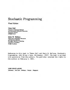
2. Problem Statement and Model When aircraft failure happens, there are several strategies to recover the flight schedule back to the regular status. The basic strategies to recover the flight timetable are delay and cancellation. For aircraft rerouting problem, strategies such as aircraft swap, type substitution, reserved aircraft, and ferry can be used. In Figure 1, a small example of aircraft routings is illustrated. The grey area means aircraft A2 found failure at 07:30, and the anticipated recovery time will be 13:15. The Airline Operation Control Center (AOCC) can choose strategy to cancel flights 4 and 5; or they can just delay flights 4–7 in a row; or aircraft A1 and A2 can switch routings at 08:00 and so forth. The figure shows a classic deterministic
Mathematical Problems in Engineering aircraft schedule recovery problem, and all the rescheduled plans are generated on the premise that the recovery time of A2 is known in advance. However, the recovery time above is an expected value which is usually given by airline maintenance staff. The value barely equals the actual one, which may make the current recovery plan not satisfactory or even infeasible. For example, if at 07:30 AOCC chooses to delay flight 4 until 13:15, but when it comes to the time 13:15, aircraft A2 is not available to use yet, more delays or cancellations will be incurred. Anther situation is that A2 is ready for use earlier than 13:15; then, a more cost-saving plan might be optional. Since the new disruption information will be updated frequently, it will be time consuming to redo the whole optimization iteratively. An intuitive thought is to generate a robust recovery plan and when the random restoration time of aircraft is determined, it is still feasible and satisfactory with simple recourse decision. In this paper, the concept of stochastic aircraft recovery time is introduced, and a two-stage aircraft schedule recovery model is established. The classic two-stage stochastic fixed recourse linear model is proposed by Dantzig [19] and Beale [20]. The model is designed to choose one decision, which makes the cost of current decision and the expectation of future recourse cost minimized [21]. For flight recovery problem, the two-stage model can evaluate the influences of different rescheduled plans and the uncertainty of the disruption factors, thereby making robust decisions. In our model, the first stage model is the deterministic resource assignment model of ARP. Based on different stochastic scenarios of aircraft recovery time, the recourse model will adjust the recovery plan obtained in the first stage. The strategy of recourse model is retiming the flights but maintaining aircraft routings generated in the first stage. It ensures the feasibility of recourse model and the simple linear formulation can guarantee the computational speed. Cancellation and aircraft swap can also be implemented as strategies in recourse model, but they will not change the essence of the model. 2.1. Stochastic Model. In the research of deterministic aircraft recovery problem, resource assignment model is one of the most prevalent ones because it can describe the problem in a complete and concise way. Our first stage model is referred to Arg¨uello et al.’s model [2]. Flights are implicitly generated as routings which will be assigned to aircraft. The notions are defined as follows: (1) Sets are as follows: 𝐹: flight set, indexed by 𝑖. 𝐾: available aircraft set, indexed by 𝑘. 𝐴: airport set, indexed by 𝑎. 𝑃: feasible aircraft routing set, indexed by 𝑗. (2) Parameters are as follows: 𝑎𝑖,𝑗 : equal to 1 if flight 𝑖 is in aircraft routing 𝑗, otherwise, equal to 0. 𝑏𝑗,𝑎 : equal to 1 if aircraft routing 𝑗 will end at airport 𝑎, otherwise, equal to 0.
Mathematical Problems in Engineering 08:00
10:00
3 12:00
14:00
16:00
18:00
20:00
22:00 T
2: BBB-CCC
1: AAA-BBB
A1
4: AAA-DDD
A2
3: CCC-AAA
6: AAA-EEE
5: DDD-AAA
7: EEE-AAA
Aircraft recovery time
Figure 1: A small case of aircraft routings.
𝑐𝑖 : the cancellation cost of flight 𝑖. ℎ𝑎 :, the required amount of aircraft at airport 𝑎, at the end of recovery process. 𝑑𝑗𝑘 : the delay cost of assigning aircraft 𝑘 to routing 𝑗. (3) Decision variables are as follows: 𝑥𝑗𝑘 : equal to 1 if aircraft 𝑘 is assigned to routing 𝑗, otherwise, equal to 0. 𝑦𝑖 : equal to 1 if flight 𝑖 is cancelled, otherwise, equal to 0. Using the above notations, the first stage resource assignment model for aircraft recovery problem is min
𝑍 = ∑ ∑ 𝑑𝑗𝑘 𝑥𝑗𝑘 + ∑𝑐𝑖 𝑦𝑖
(1)
∑ ∑ 𝑎𝑖,𝑗 𝑥𝑗𝑘 + 𝑦𝑖 = 1,
(2)
𝑘∈𝐾 𝑗∈𝑃
s.t.
𝑖∈𝐹
∀𝑖 ∈ 𝐹
𝑘∈𝐾 𝑗∈𝑃
∑ ∑ 𝑏𝑗𝑎 𝑥𝑗𝑘 ≥ ℎ𝑎 ,
∀𝑎 ∈ 𝐴
𝑘∈𝐾 𝑗∈𝑃
(3)
∑ 𝑥𝑗𝑘 = 1,
∀𝑘 ∈ 𝐾
(4)
𝑥𝑗𝑘 = 0, 1,
∀ (𝑗, 𝑘) ∈ 𝑃 × 𝐾
(5)
𝑦𝑖 = 0, 1,
∀𝑖 ∈ 𝐹.
(6)
𝑗∈𝑃
The objective function (1) minimizes the cost of flight delay and cancellation. Constraints (2) are flight coverage constraints. For any flight 𝑖, it either be cancelled or assigned to a routing. Constraints (3) are aircraft balance constraints, which require certain amount of aircraft in different airports at the end of recovery process to preserve the future regular operation. Constraints (4) confine that each aircraft can only be assigned to one routing. Constraints (5) and (6) are nonnegative constraints for decision variables. The deterministic model has an underlying work: the aircraft routings are already generated on the premise that
aircraft recovery time is fixed. However, as we mentioned above, it is hard to determine the time in real operation. The research on aircraft reliability and maintainability [22] also supports this point of view. Therefore, an expected cost that is incurred by stochasticity is added to the optimization model; it reflects the possible changes of the rescheduled plans in the first stage. The general stochastic model formulation is as follows: RP = min 𝑊 = min s.t.
(𝑍 + Q (𝑥, 𝑦))
(7)
A [𝑥, 𝑦] = b
(8)
𝑥, 𝑦 = 0, 1.
(9)
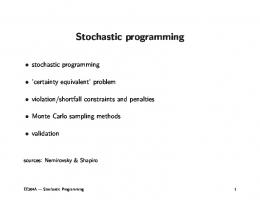
The objective function (7) of the stochastic model consists of two parts. The first one is the objective function (1); the second one Q(𝑥, 𝑦) is the expected cost of the future recourse decision on the rescheduled plans obtained at the first stage. Here, and in the following text, 𝑥 and 𝑦 are the simplified symbols which denote 𝑥𝑗𝑘 and 𝑦𝑖 in the deterministic model, respectively. Formula (8) is the general form of constraints (2)–(4). Constraints (9) are the nonnegative constraints. It is a standard two-stage recourse stochastic integer programming model. 2.2. Recourse Model. Since operations of flight schedule weave so many resources together, frequent severe changes on recovery plan are not preferred. Thus, it is meaningful to get a flexible, robust but also cost-saving recovery plan when disruption happens. Particularly, as the time passes, when the uncertain variables are determined, the selected rescheduled plan in the first stage can be implemented smoothly with or without minor adjustments. To obtain such rescheduled plan quickly is more acceptable than simply the pursuit of optimal solution in deterministic model of NP-Hard problem. Figure 2 illustrates one rescheduled plan obtained in the first stage model from the same example in Figure 1. It swaps aircraft routings of aircraft A1 and A2 and delayed the flights 1–3. Obviously, the plan is drawn on the given aircraft recovery time, which is the end of the grey interval. In reality, the A2 recovery time may be a random variable with
4
Mathematical Problems in Engineering
ΔT 08:00
10:00
12:00
PDF of recovery time of A2 14:00
16:00
18:00
20:00
22:00
24:00 T
A1
5: DDD-AAA
4: AAA-DDD
6: AAA-EEE 1: AAA-BBB
A2
7: EEE-AAA 3: CCC-AAA
2: BBB-CCC
Expected restoration time of A2
Figure 2: Illustration on recovery time of aircraft and recovery plan.
probability density function (PDF) curve in the figure, and its range is ∇𝑇. If A2 turns out to be ready at 14:00, then flights 1– 3 will be redelayed in a row; if the new arrival time of flight 3 is beyond the curfew time of airport AAA, it will be cancelled, which will break the aircraft balance also; or it will be delayed until the curfew time is over, which will impose severe delay to the flight. This situation will be reflected in terms of risk cost in the recourse model. The deterministic aircraft schedule recovery problem is an NP-hard problem; so no algorithm can be proved to be capable of obtaining optimality in polynomial time. A quick recovery solution is preferred and sometimes required. For two-stage stochastic model, there are a bunch of recourse models to be solved on each feasible solution obtained in the first stage. It requires the recourse model to be simple to solve. Let T denote the aircraft recovery time vector. It consists of every disrupted aircraft recovery time, which is considered as a continuous variable, and every available time for undisrupted aircraft which is a constant variable. Then, the objective function of the recourse model can be modeled as Q(𝑥, 𝑦) = ∫ Q(𝑥, 𝑦, T)dT. Since the objective function is nonlinear and the PDF of the random variable is usually hard to obtain as well, we can discretize the aircraft recovery time without losing precision. The combinations of discretized points from every aircraft construct the finite scenario set Ω. Let 𝜔 ∈ Ω denote one scenario (combination), and Pr(𝜔) is the probability of 𝜔. The recourse cost of the rescheduled plan can be expressed in the following: Q (𝑥, 𝑦) = ∑Q (𝑥, 𝑦, 𝜔) Pr (𝜔) . 𝜔
𝜑𝑖 : cost of breaking curfew regulation of flight 𝑖. 𝑔𝑘 : minimum turnaround time of aircraft 𝑘.
𝑡𝜔𝑘 : recovery/ready time of aircraft 𝑘 under scenario 𝜔; so the random vector 𝜉(𝜔) = (𝑡𝜔𝑘 , 𝑘 = 1, . . . , |𝐾|). Δ 𝑖 : delay time of flight 𝑖 obtained from optimization on the first stage. 𝑝(𝑖): predecessor flight of flight 𝑖 in the same aircraft routing after optimization on the first stage.
(2) Decision variables are as follows: 𝑑𝑖,𝜔 : new estimated time of departure of flight 𝑖 under scenario 𝜔. 𝑟𝑖,𝜔 : new estimated time of arrival of flight 𝑖 under scenario 𝜔. Δ 𝑖,𝜔 : estimated delay time of flight 𝑖 under scenario 𝜔. V𝑖,𝜔 : equal to 1 if flight 𝑖 violates the curfew requirement under scenario 𝜔, otherwise, equal to 0. The recourse model can be established as follows: min
(1) Parameters are as follows: 𝑡𝑖 : fly time of flight 𝑖. 𝜌𝑖 : unit delay cost of flight 𝑖 (per minute). 𝑑𝑖s : original scheduled time of departure of flight 𝑖. 𝑑(𝑖): departure airport of flight 𝑖. 𝑟(𝑖): arrival airport of flight 𝑖. 𝑡𝑎 : starting time of curfew on airport 𝑎.
𝜔
(11)
(10)
Besides notions in the first stage model, some other notions used in recourse model are listed as follows:
Q = ∑Q (𝑥, 𝑦, 𝜔) Pr (𝜔) = ∑ (∑𝜌𝑖 (Δ 𝑖𝜔 − Δ 𝑖 ) + 𝜑𝑖 V𝑖,𝜔 ) Pr (𝜔) 𝜔
s.t.
𝑖
𝑟𝑖,𝜔 = 𝑑𝑖,𝜔 + 𝑡𝑖 ,
∀𝑖 ∈ 𝐹, ∀𝜔 ∈ Ω
𝑑𝑖,𝜔 − 𝑑𝑖s = Δ 𝑖,𝜔 ,
∀𝑖 ∈ 𝐹, ∀𝜔 ∈ Ω
𝑑𝑖,𝜔 ≥ 𝑡𝜔𝑘 ∑ 𝑎𝑖,𝑗 𝑥𝑗𝑘 , 𝑗∈𝑃
(12)
∀ (𝑖, 𝑘) ∈ 𝐹 × 𝐾, ∀𝜔 ∈ Ω (13)
𝑑𝑖,𝜔 − 𝑟𝑝(𝑖),𝜔 ≥ 𝑔𝑘 ∑ 𝑎𝑖,𝑗 𝑥𝑗𝑘 , 𝑗∈𝑃
(14) ∀ (𝑖, 𝑘) ∈ 𝐹 × 𝐾, ∀𝜔 ∈ Ω
Mathematical Problems in Engineering V𝑖,𝜔:𝑑𝑖,𝜔 ≥𝑡𝑑(𝑖) ‖𝑟𝑖,𝜔 ≥𝑡𝑟(𝑖) ≥ 1,
∀𝑖 ∈ 𝐹, ∀𝜔 ∈ Ω
V𝑖,𝜔:𝑑𝑖,𝜔