Multistage Stochastic Programming: A Scenario Tree Based Approach ...

Multistage Stochastic Programming: A Scenario Tree Based Approach to Planning under Uncertainty Boris Defourny, Damien Ernst, and Louis Wehenkel University of Li`ege, Systems and Modeling, B28, B-4000 Li`ege, Belgium {Boris.Defourny,dernst,L.Wehenkel}@ulg.ac.be

Abstract. In this chapter, we present the multistage stochastic programming framework for sequential decision making under uncertainty and stress its differences with Markov Decision Processes. We describe the main approximation technique used for solving problems formulated in the multistage stochastic programming framework, which is based on a discretization of the disturbance space. We explain that one issue of the approach is that the discretization scheme leads in practice to ill-posed problems, because the complexity of the numerical optimization algorithms used for computing the decisions restricts the number of samples and optimization variables that one can use for approximating expectations, and therefore makes the numerical solutions very sensitive to the parameters of the discretization. As the framework is weak in the absence of efficient tools for evaluating and eventually selecting competing approximate solutions, we show how one can extend it by using machine learning based techniques, so as to yield a sound and generic method to solve approximately a large class of multistage decision problems under uncertainty. The framework and solution techniques presented in the chapter are explained and illustrated on several examples. Along the way, we describe notions from decision theory that are relevant to sequential decision making under uncertainty in general.

1

INTRODUCTION

This chapter addresses decision problems under uncertainty for which complex decisions can be taken in several successive stages. By complex decisions, it is meant that the decisions are structured by numerous constraints or lie in highdimensional spaces. Problems where this situation arises include capacity planning, production planning, transportation and logistics, financial management, and others (Wallace & Ziemba, 2005). While those applications are not currently mainstream domains of research in artificial intelligence, where many achievements have already been obtained for control problems with a finite number of actions and for problems where the uncertainty is reduced to some independent noise perturbing the dynamics of the controlled system, the interest for applications closer to operations research — where single instantaneous decisions may already be hard to find and where uncertainties from the environment may be delicate to model — and for applications closer to those addressed in decision theory — where complex objectives and potentially conflicting requirements have

2

to be taken into account — seems to be growing in the machine learning community, as indicated by a series of advances in approximate dynamic programming motivated by such applications (Powell, 2007; Cs´aji & Monostori, 2008). Computing strategies involving complex decisions calls for optimization techniques that can go beyond the simple enumeration and evaluation of the possible actions of an agent. Multistage stochastic programming, the approach presented in this chapter, relies on mathematical programming and probability theory. It has been recognized by several industries — mainly in energy (Kallrath, Pardalos, Rebennack, & Scheidt, 2009) and finance (Dempster, Pflug, & Mitra, 2008) — as a promising framework to formulate complex problems under uncertainty, exploit domain knowledge, use risk-averse objectives, incorporate probabilistic and dynamical aspects, while preserving structures compatible with large-scale optimization techniques. Even for readers primarily concerned by robotics, the development of these techniques for sequential decision making under uncertainty is interesting to follow: Puterman (1994), citing Arrow (1958) on the early roots of sequential decision processes, recalls the role of the multi-period inventory models from the industry in the development of the theory of Markov Decision Processes (Chapter 3 of this book); we could also mention the role of applications in finance as a motivation for the early theory of multi-armed bandits and for the theory of sequential prediction, now an important field of research in machine learning. The objective of the chapter is to provide a functional view of the concepts and methods proper to multistage stochastic programming. To communicate the spirit of the approach, we use examples that are short in their description. We use the freely available optimization software cvx (Grant & Boyd, 2009), which has the merit of enabling occasional users of optimization techniques to conduct their own numerical experiments in Matlab (The MathWorks, Inc., 2004). We cover our recent contributions on scenario tree selection and out-ofsample validation of optimized models (Defourny, Ernst, & Wehenkel, 2009), which suggest partial answers to issues concerning the selection of approximations/discretization of multistage stochastic programs, and to issues concerning the efficient comparison among those approximations. Many details relative to optimization algorithms and specific problem classes have been left aside in our presentation. A more extensive coverage of these aspects can be found in J. Birge and Louveaux (1997); Shapiro, Dentcheva, and Ruszczy´ nski (2009). These excellent sources also present many examples of formulations of stochastic programming models. Note, however, that there is no such thing as a general theory on multistage stochastic programming that would allow the many approximation/discretization schemes proposed in the technical literature (referenced later in the chapter) to be sorted out. Background Now, even if we insist on concepts, our presentation cannot totally escape from the fact that multistage stochastic programming uses optimization techniques from mathematical programming, and can harness advances in the field of optimization. To describe what a mathematical program is, simply say that there is a function F , called the objective function, that assigns to x ∈ X a real-valued

3

cost F (x), that there exists a subset C of X, called the feasibility set, describing admissible points x (by functional relations, not by enumeration), and that the program formulates our goal of computing the minimal value of F on C, written minC F , and a solution x∗ ∈ C attaining that optimal value, that is, F (x∗ ) = minC F . Note that the set of points x ∈ C such that F (x) = minC F , called the optimal solution set and written argminC F , need not be a singleton. Obviously, many problems can be formulated in that way, and what makes the interest of optimization theory is the clarification of the conditions on F and C that make a minimization problem well-posed (minC F finite and attained) and efficiently solvable. For instance, in the chapter, we speak of convex optimization problems. To describe this class, imagine a point x¯ ∈ C, and assume that for each x ∈ C in a neighborhood of x ¯, we have F (x) ≥ F (¯ x). The class of convex problems is a class for which any such x ¯ belongs to the optimal solution set argminC F . In particular, the minimization of F overP C with F an affine function of x ∈ Rn n (meaning that F has values F (x) = i=1 ai xi + a0 ) and C = {x : gi (x) ≤ 0, hj (x) = 0 for i ∈ I, j ∈ J} for some index sets I, J and affine functions gi , hj , turns out to be a convex problem (linear programming) for which huge instances — in terms of the dimension of x and the cardinality of I, J — can be solved. Typically, formulation tricks are used to compensate the structural limitations on F , C by an augmentation of the dimension of x and the introduction of new constraints gi (x) ≤ 0, hj (x) = 0. For example, minimizing the piecewise linear function f (x) = max{ai x + bi : i ∈ I} defined on x ∈ R, with I = {1, . . . , m} and ai , bi ∈ R, is the same as minimizing the linear function F (x, t) = t over the set C = {(x, t) ∈ R × R : ai x + bi − t ≤ 0, i ∈ I}. The trick can be particularized to f (x) = |x| = max{x, −x}. For more on applied convex optimization, we refer to Boyd and Vandenberghe (2004). But if the reader is ready to accept that conditions on F and C form well-characterized classes of problems, and that through some modeling effort one is often able to formulate interesting problems as an instance of one of those classes, then it is possible to elude a full description of those conditions. Stochastic programming (Dantzig, 1955) is particular from the point of view of approximation and numerical optimization in that it involves a representation of the objective F by an integral (as soon as F stands for an expected cost under a continuous probability distribution), a large, possibly infinite number of dimensions for x, and a large, possibly infinite number of constraints for defining the feasibility set C. In practice, one has to work with approximations F 0 , C 0 , and be content with an approximate solution x0 ∈ argminC 0 F 0 . Multistage stochastic programming (the extension of stochastic programming to sequential decision making) is challenging in that small imbalances in the approximation can be amplified from stage to stage, and that x0 may be lying in a space of dimension considerably smaller than the initial space for x. Special conditions might be required for ensuring the compatibility of an approximate solution x0 with the initial requirement x ∈ C. One of the main messages of the chapter is that it is actually possible to make use of supervised learning techniques (Hastie, Tibshirani, & Friedman, 2009) to lift x0 to a full-dimensional approximate solution x ˜ ∈ C, and then use an estimate of the value F (˜ x) as a feedback signal on the quality of the approximation of F , C by F 0 , C 0 .

4

The computational efficiency of this lifting procedure based on supervised learning allows us to compare reliably many approximations of F and C, and therefore to sort out empirically, for a given problem or class of problems at hand, the candidate rules that are actually relevant for building better approximations. This new methodology for guiding the development of discretization procedures for multistage stochastic programming is exposed in the present chapter. We recall that supervised learning aims at generalizing a finite set of examples of input-output pairs, sampled from an unknown but fixed distribution, to a mapping that predicts the output corresponding to a new input. This can be viewed as the problem of finding parameters maximizing the likelihood of the observed pairs (if the mapping has a parametric form); alternatively this can be viewed as the problem of selecting, from a hypothesis space of controlled complexity, the hypothesis that minimizes the expectation of the discrepancy between true outputs and predictions, measured by a certain loss function. The complexity of the hypothesis space is determined by comparing the performance of learned predictors on unseen input samples. Common methods for tackling the supervised learning problem include: neural networks (Hinton, Osindero, & Teh, 2006), support vector machines (Steinwart & Christman, 2008), Gaussian processes (Rasmussen & Williams, 2006), and decision trees (Breiman, Friedman, Stone, & Olshen, 1984; Geurts, Ernst, & Wehenkel, 2006). A method may be preferable to another depending on how easily one can incorporate prior knowledge in the learning algorithm, as this can make the difference between rich or poor generalization abilities. Note that supervised learning is integrated to many approaches for tackling the reinforcement learning problem (Chapter 4 of this book). The literature on this aspect is large: see, for instance, Lagoudakis and Parr (2003); Ernst, Geurts, and Wehenkel (2005); Langford and Zadrozny (2005); Munos and Szepesv´ari (2008). Organization of the Chapter The chapter is organized as follows. We begin by presenting the multistage stochastic programming framework, the discretization techniques, and the considerations on numerical optimization methods that have an influence on the way problems are modeled. Then, we compare the approach to Markov Decision Processes, discuss the curse of dimensionality, and put in perspective simpler decision making models based on numerical optimization, such as two-stage stochastic programming with recourse or Model Predictive Control. Next, we explain the issues posed by the dominant approximation/discretization approach for solving multistage programs (which is suitable for handling both discrete and continuous random variables). A section is dedicated to the proposed extension of the multistage stochastic programming framework by techniques from machine learning. The proposal is followed by an extensive case study, showing how the proposed approach can be implemented in practice, and in particular how it allows to infer guidelines for building better approximations of a particular problem at hand. The chapter is complemented by a discussion of issues arising from the choice of certain objective functions that can lead to inconsistent sequences of decisions, in a sense that we will make precise. The conclusion indicates some avenues for future research.

5

2

THE DECISION MODEL

This section describes the multistage stochastic programming approach to sequential decision making under uncertainty, starting from elementary considerations. The reader may also want to take a look at the example at the end of this section (and to the few lines of Matlab code that implement it). 2.1

From Nominal Plans to Decision Processes

In their first attempt towards planning under uncertainty, decision makers often set up a course of actions, or nominal plan (reference plan), deemed to be robust to uncertainties in some sense, or to be a wise bet on future events. Then, they apply the decisions, often diverging from the nominal plan to better take account of actual events. To further improve the plan, decision makers are then led to consider (i) in which parts of the plan flexibility in the decisions may help to better fulfill the objectives, and (ii) whether the process by which they make themselves (or the system) “ready to react” impacts the initial decisions of the plan and the overall objectives. If the answer to (ii) is positive, then it becomes valuable to cast the decision problem as a sequential decision making problem, even if the net added value of doing so (benefits minus increased complexity) is unknown at this stage. During the planning process, the adaptations (or recourse decisions) that may be needed are clarified, their influence on prior decisions is quantified. The notion of nominal plan is replaced by the notion of decision process, defined as a course of actions driven by observable events. As distinct outcomes have usually antagonist effects on ideal prior decisions, it becomes crucial to determine which outcomes should be considered, and what importance weights should be put on these outcomes, in the perspective of selecting decisions under uncertainty that are not regretted too much after the dissipation of the uncertainty by the course of real-life events. 2.2

Incorporating Probabilistic Reasoning

In the robust optimization approach to decision making under uncertainty, decision makers are concerned by worst-case outcomes. Describing the uncertainty is then essentially reduced to drawing the frontier between events that should be considered and events that should be excluded from consideration. In that context, outcomes under consideration form the uncertainty set, and decision making becomes a game against some hostile opponent that selects the worst outcome from the uncertainty set. The reader will find in Ben-Tal, El Ghaoui, and Nemirovski (2009) arguments in favor of robust approaches. In a stochastic programming approach, decision makers use a softer frontier between possible outcomes, by assigning weights to outcomes and optimizing some aggregated measure of performance that takes into account all these possible outcomes. In that context, the weights are often interpreted as a probability measure over the events, and a typical way of aggregating the events is to consider the expected performance under that probability measure. Furthermore, interpreting weights as probabilities allows reasoning under uncertainty. Essentially, probability distributions are conditioned on observations, and Bayes’ rule from probability theory (Chapter 2 of this book) quantifies how decision makers’ initial beliefs about the likelihood of future events — be it

6

from historical data or from bets — should be updated on the basis of new observations. Technically, it turns out that the optimization of a decision process contingent to future events is more tractable (read: suitable to large-scale operations) when the “reasoning under uncertainty” part can be decoupled from the optimization process itself. Such a decoupling occurs in particular when the probability distributions describing future events are not influenced in any way by the decisions selected by the agent, that is, when the uncertainty is exogenous to the decision process. Examples of applications where the uncertainty can be treated as an exogenous process include capacity planning (especially in the gas and electricity industries), and asset and liability management. In both case, historical data allows to calibrate a model for the exogenous process. 2.3

The Elements of the General Decision Model

We are now in a position to describe the general decision model used throughout the chapter, and introduce some notations. The model is made of the following elements. 1. A sequence of random variables ξ1 , ξ2 , . . . , ξT defined on a probability space (Ω, B, P). For a rigorous definition of the probability space, see e.g. Billingsley (1995). We simply recall that for a real-valued random variable ξt , interpreted, in the context of the rigorous definition of the probability space, as a B-measurable mapping from Ω to R with values ξt (ω), the probability that ξt ≤ v, written P{ξt ≤ v}, is the measure under P of the set {ω ∈ Ω : ξt (ω) ≤ v} ∈ B. One can write P (ξt ≤ v) for P(ξt ≤ v) when the measure P is clear from the context. If ξ1 , . . . , ξT are real-valued random variables, the function of (v1 , . . . , vT ) with values P{ξ1 ≤ v1 , . . . , ξT ≤ vT } is the joint distribution function of ξ1 , . . . , ξT . The smallest closed set Ξ in RT such that P{(ξ1 , . . . , ξT ) ∈ Ξ} = 1 is the support of measure P of (ξ1 , . . . , ξT ), also called the support of the joint distribution. If the random variables are vector-valued, the joint distribution function can be defined by breaking the random variables into their scalar components. For simplicity, we may assume that the random variables have a joint density (with respect the Lebesgue measure for continuous random variables, or with respect to the counting measure for discrete random variables), written P(ξ1 , . . . , ξT ) by a slight abuse of notation, or p(ξ1 , . . . , ξT ) if the measure P can be understood from the context. As several approximations to P are introduced in the sequel and compared to the exact measure P, we always stress the appropriate probability measure in the notation. The random variables represent the uncertainty in the decision problem, and their possible realizations (represented by the support of measure P) are the possible observations to which the decision maker will react. The probability measure P serves to quantify the prior beliefs about the uncertainty. There is no restriction on the structure of the random variables; in particular, the random variables may be dependent. When the realization of ξ1 , . . . , ξt−1 is known, there is a residual uncertainty represented by the random variables ξt , . . . , ξT , the distribution of which in now conditioned on the realization of ξ1 , . . . , ξt−1 .

7 Table 1. Decision stages, setting the order of observations and decisions. Stage

Available information for taking decisions Prior decisions

1 2 3 .. . T optional: T +1

Observed outcomes

Decision

Residual uncertainty

none u1 u1 , u2

none ξ1 ξ1 , ξ2

P(ξ1 , . . . , ξT ) P(ξ2 , . . . , ξT | ξ1 ) P(ξ3 , . . . , ξT | ξ1 , ξ2 )

u1 , . . . , uT −1

ξ1 , . . . , ξT −1

P(ξT | ξ1 , . . . , ξT −1 )

u1 u2 u3 .. . uT

u1 , . . . , uT

ξ1 , . . . , ξ T

none

(uT +1 )

For example, the evolution of the price of resources over a finite time horizon T can be represented, in a discrete-time model, by a random process ξ1 , . . . ξT , with the dynamics of the process inferred from historical data. 2. A sequence of decisions u1 , u2 , . . . , uT defining the decision process for the problem. Some models also use a decision uT +1 . We will assume that ut is valued in a Euclidian space Rm (the space dimension m, corresponding to a number of scalar decisions, could vary with the index t, but we will not stress that in the notation). For example, a decision ut could represent quantities of resources bought at time t. 3. A convention specifying when decisions should actually be taken and when the realizations of the random variables are actually revealed. This means that if ξt−1 is observed before taking a decision ut , we can actually adapt ut to the realization of ξt−1 . To this end, we identify decision stages: see Table 1. A row of the table is read as follows: at decision stage t > 1, the decisions u1 , . . . , ut−1 are already implemented (no modification is possible), the realization of the random variables ξ1 , . . . , ξt−1 is known, the realization of the random variables ξt , . . . , ξT is still unknown but a density P(ξt , . . . , ξT | ξ1 , . . . , ξt−1 ) conditioned on the realized value of ξ1 , . . . , ξt−1 is available, and the current decision to take concerns the value of ut . Once such a convention holds, we need not stress in the notation the difference between random variables ξt and their realized value, or decisions as functions of uncertain events and the actual value for these decisions: the correct interpretation is clear from the context of the current decision stage. The adaptation of a decision ut to prior observations ξ1 , . . . , ξt−1 will always be made in a deterministic fashion, in the sense that ut is uniquely determined by the value of (ξ1 , . . . , ξt−1 ). A sequential decision making problem has more than two decision stages inasmuch as the realizations of the random variables are not revealed simultaneously: the choice of the decisions taken between successive observations has to take into account some residual uncertainty on future observations. If the realization of several random variables is revealed before actually taking a decision, then the corresponding random variables should be merged into a single random vector; if several decisions are taken without intermediary ob-

8

servations, then the corresponding decisions should be merged into a single decision vector. This is how a problem concerning several time periods could actually be a two-stage stochastic program, involving two large decision vectors u1 (first-stage decision, constant), u2 (recourse decision, adapted to the observation of ξ1 ). What is called a decision in a stochastic programming model may thus actually correspond to several actions implemented over a certain number of discrete time periods. 4. A sequence of feasibility sets U1 , . . . , UT describing which decisions u1 , . . . , uT are admissible. When ut ∈ Ut , one says that ut is feasible. The feasibility sets U2 , . . . , UT may depend, in a deterministic fashion, on available observations and prior decisions. Thus, following Table 1, Ut may depend on ξ1 , u1 , ξ2 , u2 , . . . , ξt−1 in a deterministic fashion. Note that prior decisions are uniquely determined by prior observations, but for convenience we keep track of prior decisions to parameterize the feasibility sets. An important role of the feasibility sets is to model how decisions are affected by prior decisions and prior events. In particular, a situation with no possible recourse decision (Ut empty at stage t, meaning that no feasible decision ut ∈ Ut exists) is interpreted as a catastrophic situation to be avoided at any cost. We will always assume that the planning agent knows the set-valued mapping from the random variables ξ1 , . . . , ξt−1 and the decisions u1 , . . . , ut−1 to the set Ut of feasible decisions ut . We will also assume that the feasibility sets are such that a feasible sequence of decisions u1 ∈ U1 , . . . , uT ∈ UT exists for all possible joint realizations of ξ1 , . . . , ξT . In particular, the fixed set U1 must be nonempty. A feasibility set Ut parameterized only by variables in a subset of {ξ1 , . . . , ξt−1 } must be nonempty for any possible joint realization of those variables. A feasibility set Ut also parameterized by variables in a subset of {u1 , . . . , ut−1 } must be implicitly taken into account in the definition of the prior feasibility sets, so as to prevent immediately a decision maker from taking a decision at some earlier stage that could lead to a situation at stage t with no possible recourse decision (Ut empty), be it for all possible joint realizations of the subset of {ξ1 , . . . , ξt−1 } on which Ut depends, or for some possible joint realization only. These implicit requirements will affect in particular the definition of U1 . For a technical example, interpret a ≥ b for any vectors a, b ∈ Rq as a shorthand for the componentwise inequalities ai ≥ bi , i = 1, . . . , q, assume that ut−1 , ut ∈ Rm , and take Ut = {ut ∈ Rm : ut ≥ 0, At−1 ut−1 + Bt ut = ht (ξt−1 )} with At−1 , Bt ∈ Rq×m fixed matrices, and ht an affine function of ξt−1 with values in Rq . If Bt is such that {Bt ut : ut ≥ 0} = Rq , meaning that for any v ∈ Rq , there exists some ut ≥ 0 with Bt ut = v, then this is true in particular for v = ht (ξt−1 ) − At−1 ut−1 , so that Ut is never empty. More details on this kind of sufficient conditions in the stochastic programming literature can be found in Wets (1974). One can use feasibility sets to represent, for instance, the dynamics of resource inflows and outflows, assumed to be known by the planning agent. 5. A performance measure, summarizing the overall objectives of the decision maker, that should be optimized. It is assumed that the decision maker knows the performance measure. In this chapter, we write the performance measure as the expectation of a function f that assigns some scalar value to

9

each realization of ξ1 , . . . , ξT and u1 , . . . , uT , assuming the integrability of f with respect to the joint distribution of ξ1 , . . . , ξT . P For example, one could take for f a sum of scalar products Tt=1 ct · ut , where c1 is fixed and where ct depends affinely on ξ1 , . . . , ξt−1 . The function f would represent a sum of instantaneous costs over the planning horizon. The decision maker would be assumed to know the vector-valued mapping from the random variables ξ1 , . . . , ξt−1 to the vector ct , for each t. Besides the expectation, more sophisticated ways to aggregate the distribution of f into a single measure of performance have been investigated (Pflug & R¨ omisch, 2007). An important element considered in the choice of the performance measure is the tractability of the resulting optimization problem. The planning problem is then formalized as a mathematical programming problem. The formulation relies on a particular representation of the random process ξ1 , . . . , ξT in connection with the decision stages, commonly referred to as the scenario tree. 2.4

The Notion of Scenario Tree

Let us call scenario an outcome of the random process ξ1 , . . . , ξT . A scenario tree is an explicit representation of the branching process induced by the gradual observation of ξ1 , . . . , ξT , under the assumption that the random variables have a discrete support. It is built as follows. A root node is associated to the first decision stage and to the initial absence of observations. To the root node are connected children nodes associated to stage 2, one child node for each possible outcome of the random variable ξ1 . Then, to each node of stage 2 are connected children nodes associated to stage 3, one for each outcome of ξ2 given the observation of ξ1 relative to the parent node. The branching process construction goes on until the last stage is reached; at this point, the outcomes associated to the nodes on the unique path from the root to a leaf define together a particular scenario, that can be associated to the leaf. The probability distribution of the random variables is also taken into account. Probability masses are associated to the nodes of the scenario tree. The root node has probability 1, whereas children nodes are weighted by probabilities that represent the probability of the value to which they are associated, conditioned on the value associated to their ancestor node. Multiplying the probabilities of the nodes of the path from the root to a leaf gives the probability of a scenario. Clearly, an exact construction of the scenario tree would require an infinite number of nodes if the support of (ξ1 , . . . , ξT ) is discrete but not finite. A random process involving continuous random variables cannot be represented as a scenario tree; nevertheless, the scenario tree construction turns out to be instrumental in the construction of approximations to nested continuous conditional distributions. Branchings are essential to represent residual uncertainty beyond the first decision stage. At the planning time, the decision makers may contemplate as many hypothetical scenarios as desired, but when decisions are actually implemented, the decisions cannot depend on observations that are not yet available. We have seen that the decision model specifies, with decision stages, how the scenario

10

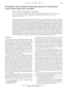
Ω

4. 1.

2.

3.

5.

1.

7. 2.

3.

8.

6.

4. 5. 6. 7. 8.

Figure 1. (From left to right) Nested partitioning of the event space Ω, starting from a trivial partition representing the absence of observations. (Rightmost) Scenario tree corresponding to the partitioning process.

actually realized will be gradually revealed. No branchings in the representation of the outcomes of the random process would mean that after conditioning on the observation of ξ1 , the outcome of ξ2 , . . . , ξT could be predicted (anticipated) exactly. Under such a representation, decisions spanning stages 2 to T would be optimized on the anticipated outcome. This would be equivalent to optimizing a nominal plan for u2 , . . . , uT that fully bets on some scenario anticipated at stage 2. To visualize how information on the realization of the random variables becomes gradually available, it is convenient to imagine nested partitions of the event space (Figure 1): refinements of the partitions appear gradually at each decision stage in correspondence with the possible realizations of the new observations. To each subregion induced by the partitioning of the event space can be associated a constant recourse decision, as if decisions were chosen according to a piecewise constant decision policy. On Figure 1, the surface of each subregion could also represent probabilities (then by convention the initial square has a unit surface and the thin space between subregions is for visual separation only). The dynamical evolution of the partitioning can be represented by a scenario tree: the nodes of the tree corresponds to the subregions of the event space, and the edges between subregions connect a parent subregion to its refined subregions obtained by one step of the recursive partitioning process. Ideally, a scenario tree should cover the totality of possible outcomes of a random process. But unless the support of the distribution of the random variables is finite, no scenario tree with a finite number of nodes can represent exactly the random process and the probability measure, as we already mentioned, while even if the support is finite, the number of scenarios grows exponentially with the number of stages. How to exploit finite scenario tree approximations in order to extract good decision policies for general multistage stochastic programming problems involving continuous distributions will be extensively addressed in this chapter. 2.5

The Finite Scenario-Tree Based Approximation

In the general decision model, the agent is assumed to have access to the joint probability distributions, and is able to derive from it the conditional distributions listed in Table 1. In practice, computational limitations will restrict the quality of the representation of P. Let us however reason at first at an abstract and ideal level to establish the program that an agent would solve for planning under uncertainty. For brevity, let ξ denote (ξ1 , . . . , ξT ), and let π(ξ) denote a decision policy mapping realizations of ξ to realizations of the decision process u1 , . . . , uT . Let

11

πt (ξ) denote ut viewed as a function of ξ. To be consistent with the decision stages, the policy must be non-anticipative, in the sense that ut cannot depend on observations relative to subsequent stages. Equivalently one can say that π1 must be a constant-valued function, π2 a function of ξ1 , and in general πt a function of ξ1 , . . . , ξt−1 for t = 2, . . . , T . The planning problem can then be stated as the search for a non-anticipative policy π, restricted by the feasibility sets Ut , that minimizes an expected total cost f spanning the decision stages and determined by the scenario ξ and the decisions π(ξ): S : minimize

E {f (ξ, π(ξ))}

subject to πt (ξ) ∈ Ut (ξ) ∀ t, π(ξ) non-anticipative .

Here we used an abstract notation which hides the nested expectations corresponding to the successive random variables, and the possible decomposition of the function f among the different decision stages indexed by t. It is possible to be even more general by replacing the expectation operator by a functional Φ assigning single numbers in R ∪ {±∞} to distributions. We also stressed the possible dependence of Ut on ξ1 , u1 , ξ2 , u2 , . . . , ξt−1 by writing Ut (ξ). A program more amenable to numerical optimization techniques is obtained by representing π(·) by a set of optimization variables for each possible argument of the function. That is, for each possible outcome ξ k = (ξ1k , . . . , ξTk ) of ξ, one associates the optimization variables (uk1 , . . . , ukT ), written uk for brevity. The non-anticipativity of the policy can be expressed by a set of equality constraints: for the first decision stage we require uk1 = uj1 for all k, j, and for subsequent k ) ≡ stages (t > 1) we require ukt = ujt for each (k, j) such that (ξ1k , . . . , ξt−1 j j (ξ1 , . . . , ξt−1 ). A finite-dimensional approximation to the program S is obtained by considering a finite number n of outcomes, and assigning to each outcome a discrete probability pk . This yields a formulation on a scenario tree covering the scenarios ξ k : Pn k k k S 0 : minimize k=1 p f (ξ , u ) subject to

uk1 = uj1

ukt ∈ Ut (ξ k ) ∀ k, ∀t ;

∀ k, j ;

ukt = ujt whenever j k (ξ1k , . . . , ξt−1 ) ≡ (ξ1j , . . . , ξt−1 )

.

Once again we used a simple notation ξ k for designating outcomes of the process ξ, which hides the fact that outcomes can share some elements according to the branching structure of the scenario tree. Non-anticipativity constraints can also be accounted for implicitly. A partial path from the root (depth 0) to some node of depth t of the scenario tree identifies k some outcome (ξ1k , . . . , ξt−1 ) of (ξ1 , . . . , ξt−1 ). To the node can be associated the k decision ut+1 , but also all decisions ujt+1 such that (ξ1k , . . . , ξtk ) ≡ (ξ1j , . . . , ξtj ). Those decisions are redundant and can be merged into a single decision on the tree, associated to the considered node of depth t (the reader may refer to the scenario tree of Figure 1).

12

The finite scenario tree approximation is needed because numerical optimization methods cannot handle directly problems like S, which cannot be specified with a finite number of optimization variables and constraints. The approximation may serve to provide an estimate of the optimal value of the original program; it may also serve to obtain an approximate first-stage decision u1 . Several aspects regarding the exploitation of scenario-tree approximations and the derivation of decisions for the subsequent stages will be further discussed in the chapter. Finally, we point out that there are alternative numerical methods for solving stochastic programs (usually two-stage programs), based on the incorporation of the discretization procedure into the optimization algorithm itself, for instance by updating the discretization or carrying out importance sampling within the iterations of a given optimization algorithm (Norkin, Ermoliev, & Ruszczy´ nski, 1998), or by using stochastic subgradient methods (Nemirovski, Juditsky, Lan, & Shapiro, 2009). Also, heuristics for finding policies directly have been suggested: a possible idea (akin to direct policy search procedures in Markov Decision Processes) is to optimize a combination of feasible non-anticipative basis policies π j (ξ) specified beforehand (Koivu & Pennanen, 2010). 2.6

Numerical Optimization of Stochastic Programs

The program formulated on the scenario tree is solved using numerical optimization techniques. In principle, it is the size, the class and the structure of the program that determine which optimization algorithm is suitable. The size depends on the number of optimization variables and the number of constraints of the program. It is therefore influenced by the number of scenarios, the planning horizon, and the dimension of the decision vectors. The class of the program depends on the range of the optimization variables (set of permitted values), the nature of the objective function, and the nature of the equality and inequality constraints that define the feasibility sets. The structure depends on the number of stages, the nature of the coupling of decisions between stages, the way random variables intervene in the objective and the constraints, and on the joint distribution of the random variables (independence assumptions or finite support assumptions can sometimes be exploited). The structure determines whether the program can be decomposed in smaller parts, and where applicable, to which extent sparsity and factorization techniques from linear algebra can alleviate the complexity of matrix operations. Note that the history of mathematical programming has shown a large gap between the complexity theory concerning some optimization algorithms, and the performance of these algorithms on problems with real-world data. A notable example (not directly related to stochastic programming, but striking enough to be mentioned here) is the traveling salesman problem (TSP). The TSP consists in finding a circuit of minimal cost for visiting n cities connected by roads (say that costs are proportional to road lengths). The dynamic programming approach, based on a recursive formulation of the problem, has the best known complexity bound: it is possible to find an optimal solution in time proportional to n2 2n . But in practice only small instances (n ∼ 20) can be solved with the algorithm developed by Bellman (1962), due to the exponential growth of a list of optimal subpaths to consider. Linear programming approaches based on the simplex

13

algorithm have an unattractive worst-case complexity, and yet such approaches have allowed to solve large instances of the problem — n = 85900 for the record on pla85900 obtained in 2006 — as explained in Applegate, Bixby, Chv´atal, and Cook (2007). In today’s state of computer architectures and optimization technologies, multistage stochastic programs are considered numerically tractable, in the sense that numerical solutions of acceptable accuracy can be computed in acceptable time, when the formulation is convex. The covered class includes linear programs (LP) and convex quadratic programs (QP), which are similar to linear programs but have a quadratic component in their objective. A problem can be recognized to be convex if it can be written as a convex program; a program minC F is convex if (i) the feasibility set C is convex, that is, (1 − λ)x + λy ∈ C whenever x, y ∈ C and 0 < λ < 1 (Rockafellar, 1970, page 10); (ii) the objective function F is convex on C, that is, F ((1 − τ )x + τ y) ≤ (1 − τ )F (x) + τ F (y), 0 < τ < 1, for every x, y ∈ C (Rockafellar, 1970, Theorem 4.1). We refer to Nesterov (2003) for an introduction to complexity theory for convex optimization and to interiorpoint methods. Integer programs (IP) and mixed-integer programs (MIP) are similar to linear programs but have integrality requirements on all (IP) or some (MIP) of their optimization variables. The research in stochastic programming for these classes is mainly focused on two-stage models: computationally-intensive methods for preprocessing programs so as to accelerate the repeated evaluation of integer recourse decisions (Schultz, Stougie, & Van der Vlerk, 1998); convex relaxations (Van der Vlerk, 2009); branch-and-cut strategies (Sen & Sherali, 2006). In large-scale applications, the modeling and numerical optimization aspects are closely integrated: see, for instance, the numerical study of Verweij, Ahmed, Kleywegt, Nemhauser, and Shapiro (2003). Solving multistage stochastic mixedinteger models is extremely challenging, but significant progress has been made recently (Escudero, 2009). In our presentation, we focus on convex problems, and use Matlab for generating the data structure and values of the scenario trees, and cvx (Grant & Boyd, 2008, 2009) for formulating and solving the resulting programs — cvx is a modeling tool: it uses a language close to the mathematical formulation of the models, leading to codes that are slower to execute but less prone to errors. 2.7

Example

To fix ideas, we illustrate the scenario tree technique on a trajectory tracking problem under uncertainty with control penalization. In the proposed example, the uncertainty is such that the exact problem can be posed on a small finite scenario tree. Say that a random process ξ = (ξ1 , ξ2 , ξ3 ), representing perturbations at time t = 1, 2, 3, has 7 possible outcomes, denoted by ξ k , 1 ≤ k ≤ 7, with known probabilities pk : k

1

2

3

4

5

6

7

ξ1k -4 -4 -4 3 3 3 3 ξ2k -3 2 2 -3 0 0 2 ξ3k 0 -2 1 0 -1 2 1 pk 0.1 0.2 0.1 0.2 0.1 0.1 0.2

14 b

b

b

2

-3 0

b b

0 -2 b

b

v2 b

v3 b

b

1 0 -1 b

b

b

b

b

b

b

b

b

b

b

b

2.1

b

2 b

2

1

x1 b

b

b

x2 b

b

b

x3

b

-1.16

0.667 1.26 -0.74

b

b

b

b

b

b

-5

0

b

b

b

-1.333 b

b

b

b

-1.26 1.74

b

b

b

2.9

b

-3

0.1 0.2 0.1 0.2 0.1 0.1 0.2

b

-4.1

-2

x4 b

0

b

b

2 b

b

b

b

3

-4 -3

-0.1

v1

b

0 b

1.667

b

3.74

b

b

3 b

0

b

b

2.74

Figure 2. (Left) Scenario tree representing the 7 possible scenarios for a random process ξ = (ξ1 , ξ2 , ξ3 ). The outcomes ξtk are written in bold, and the scenario probabilities pk are reported at the leaf nodes. (Middle) Optimal actions vt for the agent, displayed scenario per scenario, with frames around scenarios passing by a same tree node. (Right) Visited states xt under the optimal actions, treated as artificial decisions (see text).

The random process is fully represented by the scenario tree of Figure 2 (Left) — the first possible outcome is ξ 1 = (−4, −3, 0) and has probability p1 = 0.1. Note that the random variables ξ1 , ξ2 , ξ3 are not mutually independent. Assume that an agent can choose actions vt ∈ R at t = 1, 2, 3 (the notation vt instead of ut is justified in the sequel). The goal of the agent is the minimization P3 of an expected sum of costs E{ t=1 ct (vt , xt+1 ) | x1 = 0}. Here xt ∈ R is the state of a continuous-state, discrete-time dynamical system, that starts from the initial state x1 = 0 and follows the state transition equation xt+1 = xt + vt + ξt . Costs ct (vt , xt+1 ), associated to the decision vt and the transition to the state xt+1 , are defined by ct = (dt+1 + vt2 /4) with dt+1 = |xt+1 − αt+1 | and α2 = 2.9, α3 = 0, α4 = 0 (αt+1 : nominal trajectory, chosen arbitrarily; dt+1 : tracking error; vt2 /4: penalization of control effort). An optimal policy mapping observations ξ1 , . . . , ξt−1 to decisions vt can be obtained by solving the following convex quadratic program over variables vtk , xkt+1 , dkt+1 , where k runs from 1 to 7 and t from 1 to 3, and over xk1 trivially set to 0:   P3 P7 k 2 k k minimize k=1 p t=1 (dt+1 + (vt ) /4) subject to

− dkt+1 ≤ xkt+1 − αt+1 ≤ dkt+1

xk1 v11 v21 v32

=0 ,

= v12 = = v22 = = v33 ,

∀ k, t

xkt+1 = xkt + vtk + ξtk ∀ k, t v13 = v14 = v15 = v16 = v17 v23 , v24 = v25 = v26 = v27 v35 = v36 .

Here, the vector of optimization variables (v1k , xk1 ) plays the role of uk1 , the vector (vtk , xkt , dkt ) plays the role of ukt for t = 2, 3, and the vector (xk4 , dk4 ) plays the role of uk4 , showing that the decision process u1 , . . . , uT +1 of the general multistage stochastic programming model can in fact include state variables and more generally any element that serves to evaluate costs conveniently. The following code allows to formulate and solve the program using Matlab and cvx. It is almost a direct transcription of the program formulation, with variables and constraints defined in matrix form (column indices are relative to scenarios). Note that cvx replicates scalars if needed in componentwise constraints.

15

% problem data xi = [-4 -4 -4 3 3 3 3;... -3 2 2 -3 0 0 2;... 0 -2 1 0 -1 2 1]; p = [.1 .2 .1 .2 .1 .1 .2]; a = [2.9 0 0]’; x1 = 0; n = 7; T = 3; % call cvx toolbox cvx_begin variables x(T+1,n) d(T,n) v(T,n) minimize( sum(sum(d*diag(p))) ... + sum(sum((v.^2)*diag(p)))/4); subject to -d T − Q and ξt−1 > 0 . In a first experiment, we will take the numerical parameters and the process ξ selected in Hilli and Pennanen (2008) (to ease the comparisons): ρ = 1, T = 4, Q = 2; ξt = (exp{bt } − K) where K = 1 is the fixed cost (or the strike price, when the problem is interpreted as the valuation √ of an option) and bt is a random walk: b0 = σ 0 , bt = bt−1 + σ t , with σ = 0.2 and t following a standard normal distribution N (0, 1). In a second experiment over various values of the parameters (ρ, Q, T ) with T up to 52, we will take for ξ the process selected in K¨ uchler and Vigerske (2010) (because otherwise on long horizons the price levels of the first process blow out in an unrealistic way, making the problem rather trivial): ξt = (ξt0 − K) with 0 ξt0 = ξt−1 exp{σt − σ 2 /2} where σ = 0.07, K = 1, and t following a standard normal distribution. Equivalently ξt = (exp{bt − (t + 1) σ 2 /2} − K) with bt a random walk such that b0 = σ 0 and bt = bt−1 + σ t . 6.2

Algorithm for Generating Small Scenario Trees

At the heart of tree selection procedure relies our ability to generate scenario trees reduced to a very small number of scenarios, with interesting branching structures. As the trees are small, they can be solved quickly and then scored using the supervised learning policy inference procedure. Fast testing procedures make it possible to rank large numbers of random trees. The generation of random branching structures has not been explored in the classical stochastic programming literature; we thus have to propose a first algorithm in this section. The algorithm is developed with our needs in view, with the feedback provided by the final numerical results of the tests, until results on the whole set of considered numerical instances suggest that the algorithm suffices for the application at hand. We believe that the main ideas behind this algorithm will be reused in subsequent work for addressing the representation of stochastic processes of higher dimensions. Therefore, in the following explanations we put more emphasis on the methodology we followed than on the final resulting algorithm. Method of Investigation. The branching structure is generated by simulating the evolution of a branching process. We will soon describe the branching process that we have used, but observe first that the probability space behind the random generation of the tree structure is not at all related to the probability space of the random process that the tree approximates. It is the values and probabilities of the nodes that are later chosen in accordance to the target

36

probability distribution, either deterministically or randomly, using any new or existing method. For selecting the node values, we have tested different deterministic quantizations of the one-dimensional continuous distributions of random variables ξt , and alternatively different quantizations of the gaussian innovations t that serve to define ξt = ξt (t ), as described by the relations given in the previous section. Namely, we have tested the minimization of the quadratic distortion (Pages & Printems, 2003) and the minimization of the Wasserstein distance (Hochreiter & Pflug, 2007). On the considered problems we did not notice significant differences in performance attributable to a particular deterministic variant. What happened was that with deterministic methods, performances began to degrade as the planning horizon was increased, perhaps because trying to preserve statistical properties of the marginal distributions ξt distorts other statistics of the joint distribution of (ξ0 , . . . , ξT −1 ), especially in higher dimensions. Therefore, for treating instances on longer planning horizons, we switched to a crude Monte Carlo sampling for generating node values. By examining trees with the best scores in the context of the present family of problems, we observed that several statistics of the random process represented by those trees could be very far from their theoretical values, including first moments. This might suggest that it is very difficult to predict without any information on the optimal solutions which properties should be preserved in small scenario trees, and thus which objective should be optimized when attempting to build a small scenario tree. If we had discovered a correlation between some features of the trees and the scores, we could have filtered out bad trees without actually solving the programs associated to these trees, simply by computing the identified features. Description of the Branching Processes. We now describe the branching process used in the experiments made with deterministic node values. Let r ∈ [0, 1] denote a fixed probability of creating a branching. We start by creating the root node of the tree (depth 0), to which we assign the conditional probability 1. With probability r, we create 2 successor nodes to which we assign the values ±0.6745 and the conditional probabilities 0.5 (the values given here minimize the Wasserstein distance between a two mass point distribution and the standard normal distribution for t ). With probability (1 − r) we create instead a single successor node to which we assign the value 0 and the conditional probability 1; this node is a degenerate approximation of the distribution of t . Then we take each node of depth 1 as a new root and repeat the process of creating 1 or 2 successor nodes to these new roots randomly. The process is further repeated on the nodes of depth 2, . . . , T − 1, yielding a tree of depth T for representing the original process 0 , . . . , T −1 . The scenario tree for ξ is derived from the scenario tree for . For problems on larger horizons, it is difficult to keep the size of the tree under control with a single fixed branching parameter r — the number of scenarios would have a large variance. Therefore, we used a slightly more complicated branching process, by letting the branching probability r depend on the number of scenarios currently developed. Specifically, let N be a target number of scenarios and T a target depth for the scenario tree with the realizations of ξt relative to depth t + 1. Let nt be the number of parent nodes at depth t; this is a

37

random variable except at the root for which n0 = 1. During the construction of the tree, parent nodes at depth t < T are developed and split in ν = 2 children −1 nodes with a probability rt = n−1 (N −1)/T . Parent nodes have a single t (ν −1) child node with a probability 1−rt . If rt > 1, we set rt = 1 and all nodes are split −1 in ν = 2 children nodes. Thus in general rt = min{1, n−1 (N − 1)/T }. t (ν − 1) 6.3

Algorithm for Learning Policies

Solving a program on a scenario tree yields a dataset of scenario/decision sequence pairs (ξ, u). To infer a decision policy that generalizes the decisions of the tree to test scenarios, we have to learn mappings from (ξ0 , . . . , ξt−1 ) to ut and ensure the compliance of the decisions with the constraints. To some extent the procedure is thus problem-specific. Here again we insist on the methodology. Dimensionality Reduction. We try to reduce the number of features of the input space. In particular, we can try to get back to a state-action space representation of the policy (and postprocess datasets accordingly to recover the states). Note that in general needed states are those that would be used by an hypothetical reformulation of the optimization problem using dynamic programming. Here the objective is based on the exponential utility function. By the property that P E{exp{− Tt0 =1 ξt0 −1 · ut0 } | ξ0 , . . . , ξt−1 } PT Pt−1 = exp{− t0 =1 ξt0 −1 · ut0 } E{exp{− t0 =t ξt0 −1 · ut0 } | ξ0 , . . . , ξt−1 } ,

we can see that decisions at t0 = 1, . . . , t − 1 scale by a same factor the contribution to the return brought by the decisions at t0 = t, . . . , T . Therefore, if the feasibility set at time t can be expressed from state variables, the decisions at t0 = t, . . . , T can be optimized independently of the decisions at t0 = 1, . . . , t − 1. This suggests to express ut as a function of the state ξt−1 of the P process ξ, and t−1 of an additional state variable ζt defined by ζ0 := Q , ζt := Q − t0 =1 ut0 , that PT PT allows to reformulate the constraint t0 =1 ut0 ≤ Q as t0 =t ut0 ≤ ζt . Feasibility Guarantees Sought Before Repair Procedures. We try to map the output space in such a way that the predictions learned under the new geometry and then transformed back using the inverse mapping comply with the feasibility constraints. Here, we scale the output ut so as to have to learn the fraction yt = yt (ξt−1 , ζt ) of the maximal allowed output min(1, ζt ), which summarizes the two constraints of the problem. Since ζ0 = Q, we distinguish the cases u1 = y1 (ξ0 ) · 1 and ut = yt (ξt−1 , ζt ) · min(1, ζt ). It will be easy to ensure that fractions yt are valued in [0, 1] (thus we do not need to define an a posteriori repair procedure). Input Normalization. It is convenient for the sequel to normalize the inputs. From the definition of ξt−1 we can recover the state of the random walk bt−1 , and use as first input xt1 := (σ 2 t)−1/2 bt−1 , which follows a standard normal distribution. Thus for the first version of the process ξ, instead of ξt−1 we use xt1 = σ −1 t−1/2 log(ξt−1 +K), and for the second version of the process ξ, instead

38

of ξt−1 we use xt1 = σ −1 t−1/2 log(ξt−1 + K) + σt1/2 /2. Instead of the second input ζt (for t > 1) we use xt2 := ζt /Q, which is valued in [0, 1]. Therefore, we rewrite the fraction yt (ξt−1 , ζt ) as gt (xt1 , xt2 ). Hypothesis Space. We have to choose the hypothesis space for the learned fractions gt defined previously. Here we find it convenient to choose the class of feed-forward neural networks with one hidden layer of L neurons:    P2 PL gt (xt1 , xt2 ) = logsig γt + j=1 wtj · tansig βtj + k=1 vtjk xtk , with weights vtjk and wtj , biases βtj and γt , and activation functions tansig(x) = 2 · (1 + e−2 x )−1 − 1 logsig(x) = (1 + e

−x −1

)

valued in [−1, +1] , valued in [0, 1] ,

a usual choice for imposing the output ranges [−1, +1] and [0, 1] respectively. Since the training sets are extremely small, we take L = 2 for g1 (which has only one input x11 ) and L = 3 for gt (t > 1). We recall that artificial neural networks have been found to be well-adapted to nonlinear regression. Standard implementations of neural networks (construction and learning algorithms) are widely available, with a full documentation from theory to interactive demonstrations (Demuth & Beale, 1993). We report here the parameters chosen in our experiments for the sake of completeness; the method is largely off-the-shelf. Details on the Implementation. The weights and biases are determined by training the neural networks. We used the Neural Network toolbox of Matlab with the default methods for training the networks by backpropagation — the Nguyen-Widrow method for initializing the weights and biases of the networks randomly, the mean square error loss function, and the Levenberg-Marquardt optimization algorithm. We used [−3, 3] for the estimated range of xt1 , corresponding to 3 standard deviations, and [0, 1] for the estimated range of xt2 . Trained neural networks are dependent on the initial weights and biases before training, because the loss minimization problem is nonconvex. Therefore, we repeat the training 5 times from different random initializations. We obtain several candidate policies (to be ranked on the test sample). In our experiments on the problem with T = 4, we randomize the initial weights and biases of each network independently. In our experiments on problems with T > 4, we randomize the initial weights and biases of g1 (x11 ) and g2 (x21 , x22 ), but then we use the optimized weights and biases of gt−1 as the initial weights and bias for the training of gt . Such a warm-start strategy accelerates the learning tasks. Our intuition was that for optimal control problems, the decision rules πt would change rather slowly with t, at least for stages far from the terminal horizon. We do not claim that using neural networks is the only or the best way of building models gt that generalize well and are fast in exploitation mode. The choice of the Matlab implementation for the neural networks could also be criticized. It just turns out that these choices are satisfactory in terms of implementation efforts, reliability of the codes, solution quality, and overall running time.

39

6.4

Remark on Approximate Solutions

An option of the proposed testing framework that we have not discussed, as it is linked to technical aspects of numerical optimization, is that we can form the datasets of scenario/decisions pairs using inexact solutions to the optimization programs associated to the trees. Indeed, simulating a policy based on any dataset will still give a pessimistic bound on the optimal solution of the targeted problem. The tree selection procedure will implicitly take this new source of approximation into account. In fact, every approximation one can think of for solving the programs could be tested on the problem at hand and thus ultimately accepted or rejected, on the basis of the performance of the policy on the test sample, and the time taken by the solver to generate the decisions of the dataset. 6.5

Numerical Results

We now describe the numerical experiments we have carried out and comment on the results. Experiment on the small-horizon problem instance. First, we consider the process ξ and parameters (ρ, Q, T ) taken from Hilli and Pennanen (2008). We generate a sample of m = 104 scenarios drawn independently, on which each learned policy will be tested. We generate 200 random tree structures as described previously (using r = 0.5 and rejecting structures with less than 2 or more than 10 scenarios). Node values are set by the deterministic method, thus the variance in performance that we will observe among trees of similar complexity will come mainly from the branching structure. We form and solve the programs on the trees using cvx, and extract the datasets. We generate 5 policies per tree, by repeatedly training the neural networks from random initial weights and biases. Each policy is simulated on the test sample and the best of the 5 policies is retained for each tree. The result of the experiment is shown on Figure 3. Each point is relative to a particular scenario tree. Points from left to trees of P to right are PTrelative j · π ˆt (ξ j )} for increasing size. We report the value of m−1 m exp{− ξ t−1 j=1 t=1 each learned policy π ˆ , in accordance with the objective minimized in Hilli and Pennanen (2008). Lower is better. Notice the large variance of the test sample scores among trees with the same number of scenarios but different branching structures. The tree selection method requires a single lucky outlier to output a good valid upper bound on the targeted objective — quite an advantage with respect to approaches based on worst-case reasonings for building a single scenario tree. With a particular tree of 6 scenarios (best result: 0.59) we already reach the guarantee that the optimal value of our targeted problem is less or equal to log(0.59) ' −0.5276. On Figure 4, we have represented graphically some of the lucky small scenario trees associated to the best performances. Of course, tree structures that perform well here may not be optimal for other problem instances. The full experiment takes 10 minutes to run on a pc with a single 1.55 GHz processor and 512 Mb RAM. By comparing our bounds to those reported in Hilli and Pennanen (2008) — where validation experiments taking up to 30 hours with

cost of policy on the test sample

40 0.66 0.64 0.62 0.6

0.58

1

2

3

4

5

6

7

8

9 10

number of scenarios of the tree Figure 3. First experiment: scores on the test sample associated to the random scenario trees (lower is better). The linear segments join the best scores of policies inferred from trees of equivalent complexity.

1/4

+0.828 +0.352

1/8 1/4

+0.000

1/8

-0.260 -0.453

1/4

ξ0k

ξ1k

ξ2k

ξ3k

+0.828

1/4

+0.352

1/8 1/8

+0.000 1/8 1/8 1/4

-0.260 -0.453

pk

ξ0k

ξ1k

ξ2k

ξ3k

+1.472

+1.472

1/8

1/8 +0.828 1/8 1/8

+0.352 +0.000

1/4 1/8

-0.260 -0.453 -0.595

1/8 1/8

ξ0k

ξ1k

ξ2k

ξ3k

pk

pk

+0.828

1/16

+0.352

1/8 1/16 1/16 1/4 1/8 1/16 1/8

+0.000 -0.260 -0.453 -0.595

ξ0k

ξ1k

ξ2k

ξ3k

pk

Figure 4. Small trees (5,6,7,9 scenarios) from which good datasets could be obtained. The scenarios ξ k = (ξ0k , ξ1k , ξ2k ) are shifted vertically to distinguish them when they pass through common values, written on the left. Scenario probabilities pk are indicated on the right.

a single 3.8Ghz processor, 8Gb RAM have been carried out — we deduce that we reached essentially the quality of the optimal solution. Experiment on large-horizon problem instances. Second, we consider the process ξ taken from K¨ uchler and Vigerske (2010) and a series of 15 sets of parameters for (ρ, Q, T ). We repeat the following experiment on each (ρ, Q, T ) with 3 different parameter values for controlling the size of the random trees:

41 Table 2. Second experiment: Best upper bounds for a family of problem instances. Upper bounds1

Problem

ρ

0

Q T

Reference2

Value of the best policy3 , in function of N N =1·T

N =5·T

N = 25 · T

2 2 6 6 20

12 52 12 52 52

-0.1869 -0.4047 -0.5062 -1.1890 -3.6380

-0.1837 -0.3418 -0.5041 -1.0747 -3.5867

-0.1748 -0.3176 -0.4889 -1.0332 -3.5000

-0.1797 -0.3938 -0.4930 -1.1764 -3.4980

0.25 2 2 6 6 20

12 52 12 52 52

-0.1750 -0.3351 -0.4363 -0.7521 -1.4625

-0.1716 -0.3210 -0.4371 -0.7797 -1.8923

-0.1661 -0.3092 -0.4381 -0.7787 -1.9278

-0.1700 -0.3288 -0.4365 -0.8030 -1.9128

12 52 12 52 52

-0.1466 -0.2233 -0.3078 -0.3676 -0.5665

-0.1488 -0.2469 -0.3351 -0.5338 -0.9625

-0.1473 -0.2222 -0.3385 -0.5291 -0.9757

-0.1458 -0.2403 -0.3443 -0.5354 -0.9624

1

1 2 3

2 2 6 6 20

Estimated on a test sample of m = 10000 scenarios. On a same row, lower is better. Defined by πtref (ξ) and optimal for the risk-neutral case ρ = 0. On random trees of approximately N scenarios.

generate 25 random trees (we recall that this time the node values are also randomized), solve the resulting 25 programs, learn 5 policies per tree (depending on the random initialization of the neural networks), and report as the best score the lowest of the resulting 125 values computed on the test sample. Table 2 reports values corresponding to the average performance ρ−1 log{m−1

m X j=1

exp{−ρ

T X t=1

j ξt−1 ·π ˆt (ξ j )}}

obtained for a series of problem instances, the numerical parameters of which are given in the first column of the table, for different policies selected among random trees of 3 different nominal sizes, so as to investigate the effect of the size of the tree on the performance of the learned policies. One column is dedicated to the performance of the analytical reference policy π ref on the test sample. In the case ρ = 0, the reference value provided by the analytical optimal policy suggests that the best policies are close to optimality. In the case ρ = 0.25, the reference policy is now suboptimal. It still slightly dominates the learned policies when Q = 2, but not anymore when Q = 6 or Q = 20. In the case ρ = 1, the reference policy is dominated by the learned policies, except perhaps when Q = 2 and the trees are large. That smaller trees are sometimes better than large trees may be explained by the observation that multiplying the number of scenarios by 25, as done in our experiments, does not fundamentally change the order of magnitude of size of the tree, given the required exponential growth of the number of scenarios with the number of stages.

42

This experiment shows that even if the scenario tree selection method requires generating and solving several trees, rather than one single tree, it can work very well. In fact, with a random tree generation process that can generate a medium size set of very small trees, there is a good likelihood in the problem that at least one of those trees will lead to excellent performances. Large sets of scenario trees could easily be processed simply by parallelizing the tree selection procedure. Overall, the approach seems promising in terms of the usage of computational resources.

7

TIME INCONSISTENCY AND BOUNDED RATIONALITY LIMITATIONS

This section discusses the notion of dynamically consistent decision process, which is relevant to sequential decision making with risk-sensitivity — by opposition to the optimization of the expectation of a total return over the planning horizon, which can be described as risk-indifferent, or risk-neutral. 7.1

Time-Consistent Decision Processes

We will say that an objective induces a dynamically consistent policy, or timeconsistent policy, if the decisions selected by a policy optimal for that objective coincide with the decisions selected by a policy recomputed at any subsequent time step t and optimal for the same objective with decisions and observations prior to t set to their realized value (and decisions prior to t chosen according to the initial optimal policy). Time-consistent policies are not necessarily time-invariant: we simply require that the optimal mappings πt from information states it to decisions ut at time t, evaluated from some initial information state at t = 0, do not change if we take some decisions following these mappings, and then decide to recompute them from the current information state. We recall that in the Markov Decision Process framework, the information state it is the current state xt , and in the multistage stochastic programming framework, it is the current history (ξ1 , . . . , ξt−1 ) of the random process, with t indexing decision stages. We say that a decision process is time-consistent if it is generated by a time-consistent policy. A close notion of time-consistency can also be defined by saying that the preferences of the decision maker among possible distributions for the total return over the planning horizon can never be affected by future information states that the agent recognizes, at some point in the decision process, as impossible to reach (Shapiro, 2009; Defourny, Ernst, & Wehenkel, 2008). In the absence of time-consistency, the following situation may arise (the discussion is made in the multistage stochastic programming framework). At time t = 1, an agent determines that for each possible outcome of a random variable ξ2 at time t = 2, the decision u2 = a at time t = 2 is optimal (with respect to the stated objective and constraints of the problem, given the distribution of ξ2 , ξ3 , . . . , and taking account of optimized recourse decisions u3 , u4 , . . . over the planning horizon). Then at time t = 2, having observed the outcome of the random variable ξ1 and conditioned the probability distributions of ξ2 , ξ3 , . . . over this observation, and in particular, having ruled out all scenarios where ξ1 differs

43

from the observed outcome, the agent finds that for some possible realizations of ξ2 , u2 = a is not optimal. The notion of time-consistency already appears in Samuelson (1937), who states: “as the individual moves along in time there is a sort of perspective phenomenon in that his view of the future in relation to his instantaneous time position remains invariant, rather than his evaluation of any particular year” (page 160). Several economists have rediscovered and refined the notion (Strotz, 1955; Kydland & Prescott, 1977), especially when trying to apply expected utility theory, valid for comparisons of return distributions viewed from a single initial information state, to sequential decision making settings, where the information state evolves. In fact, if an objective function subject to constraints can be optimized by dynamic programming, in the sense that a recursive formulation of the optimization is possible using value functions (on an augmented state space if necessary, and irrespectively of complexity issues), then an optimal policy will satisfy the time-consistency property. This connection between Bellman’s principle (1957) and time-consistency is well-established (Epstein & Schneider, 2003; Artzner, Delbaen, Eber, Heath, & Ku, 2007). By definition and by recursion, a value function is not affected by states that have a zero probability to be reached in the future; when the value function is exploited, a decision ut depends only on the current information state it . Objectives that can be optimized recursively include the expected sum of rewards, and the expected exponential utility of a sum of rewards (Howard & Matheson, 1972), with discount permitted, although the recursion gets more involved (Chung & Sobel, 1987). A typical example of objective that cannot be rewritten recursively in general is the variance of the total return over several decision steps. This holds true even if the state fully describes the distribution of total returns conditionally to the current state. Note, however, that a nice way of handling a mean-variance objective on the total return is to relate it to the expected exponential utility: if R denotes a random total return, Φρ {R} = E{R} − (ρ/2)var{R} ' −ρ−1 log E{exp(−ρR)}. The approximation holds for small ρ > 0. It is exact for all ρ > 0 if R follows a Gaussian distribution. 7.2

Limitations of Validations Based on Learned Policies

In our presentation of multistage stochastic programming, we did not discuss several extensions that can be used to incorporate risk awareness in the decision making process. In particular, a whole branch of stochastic programming is concerned with the incorporation of chance constraints in models (Pr´ekopa, 1995), that is, constraints to be satisfied with a probability less than 1. Another line of research involves the incorporation of modern risk measures such as the conditional value-at-risk at level α (expectation of the returns relative to the worst α-quantile of the distribution of returns) (Rockafellar & Uryasev, 2000). An issue raised by many of these extensions, when applied to sequential decision making, is that they may induce time-inconsistent decision making processes (Boda & Filar, 2006). The validation techniques based on supervised learning that we have proposed are not adapted to time-inconsistent processes. Indeed, these techniques rely on the assumption that the optimal solution of a multistage stochastic program is a sequence of optimal mappings πt from reachable information states

44

(ξ1 , . . . , ξt−1 ) to feasible decisions ut , uniquely determined by some initial information state at which the optimization of the mappings takes place. We believe, however, that the inability to address the full range of possible multistage programming models should have minor practical consequences. On the one hand, we hardly see the point of formulating a sophisticated multistage model with optimal recourse decisions unrelated to those that would be implemented if the corresponding information states are actually reached. On the other hand, it is always possible to simulate any learned policy, whatever the multistage model generating the learning data might be, and score an empirical return distribution obtained with the simulated policy according to any risk measure important for the application. Computing a policy and sticking to it, even if preferences are changing over time, is a form of precommitment (Hammond, 1976). Finally, let us observe that a shrinking-horizon policy can be time-inconsistent for two reasons: (i) the policy is based on an objective that cannot induce a timeconsistent decision process; (ii) the policy is based on an objective that could be reformulated using value functions, but anyway the implicit evaluation of these value functions changes over time, due to numerical approximations local to the current information state. Similarly, if an agent uses a supervised-learning based policy to take decisions at some stage and is then allowed to reemploy the learning procedure at later stages, the overall decision sequence may appear as dynamically inconsistent. The source (ii) of inconsistency appears rather unavoidable in a context of bounded computational resources; more generally, it seems that bounded rationality (Simon, 1956) would necessarily entail dynamical inconsistency.

8

CONCLUSIONS

In this chapter, we have presented the principles of the multistage stochastic programming approach to sequential decision making under uncertainty, and discussed the inference and exploitation of decision policies for comparing various approximations of a multistage program in the absence of tight theoretical guarantees. Sequential decision making problems under uncertainty form a rich class of optimization problems with many challenging aspects. Markov Decision Processes and multistage stochastic programming are two frameworks for addressing such problems. They have been originally studied by different communities, leading to a separate development of new approximation and solution techniques. In both fields, research is done so as to extend the scope of the framework to new problem classes: in stochastic programming, there is research on robust approaches (Delage & Ye, 2008), decision-dependent random processes (Goel & Grossmann, 2006), nonconvex problems (Dentcheva & R¨ omisch, 2004); in Markov Decision Processes, many efforts are directed at scaling dynamic programming (or policy search) to problems with high-dimensional continuous state spaces and/or decision spaces (Ng & Jordan, 1999; Ghavamzadeh & Engel, 2007; Antos, Munos, & Szepesv´ari, 2008). It is likely that a better integration of the ideas developed in the two fields will ultimately yield better solving strategies for large-scale problems having both continuous and discrete aspects. Both fields have foundations in empirical process theory, and can benefit from advances in Monte Carlo methods, espe-

45

cially in variance reduction techniques (Singh, Kantas, Vo, Doucet, & Evans, 2007; Coquelin, Deguest, & Munos, 2009; Hoffman, Kueck, Doucet, & de Freitas, 2009). Acknowledgments This paper presents research results of the Belgian Network DYSCO (Dynamical Systems, Control, and Optimization), funded by the Interuniversity Attraction Poles Programme, initiated by the Belgian State, Science Policy Office. The scientific responsibility rests with its authors. Damien Ernst is a Research Associate of the Belgian FRS-FNRS of which he acknowledges the financial support. This work was supported in part by the IST Programme on the European Community, under the PASCAL2 Network of Excellence, IST-2007-216886. This publication only reflects the authors’ views.

46

References Antos, A., Munos, R., & Szepesv´ari, C. (2008). Fitted Q-iteration in continuous action-space MDPs. In Advances in Neural Information Processing Systems 20 (NIPS-2007) (p. 9-16). Cambridge, MA: MIT Press. Applegate, D. L., Bixby, R. E., Chv´atal, V., & Cook, W. J. (2007). The traveling salesman problem: A computational study. Princeton, NJ: Princeton University Press. Arrow, K. J. (1958). Historical background. In K. J. Arrow, S. Karlin, & H. Scarf (Eds.), Studies in the mathematical theory of inventory and production. Stanford, CA: Stanford University Press. Artzner, P., Delbaen, F., Eber, J.-M., Heath, D., & Ku, H. (2007). Coherent multiperiod risk adjusted values and Bellman’s principle. Annals of Operations Research, 152 (1), 5-22. Balasubramanian, J., & Grossmann, I. E. (2003). Approximation to multistage stochastic optimization in multiperiod batch plant scheduling under demand uncertainty. Industrial & Engineering Chemistry Research(43), 3695-3713. Bellman, R. (1962). Dynamic programming treatment of the travelling salesman problem. Journal of the ACM , 9 , 61-63. Ben-Tal, A., El Ghaoui, L., & Nemirovski, A. (2009). Robust optimization. Princeton, NJ: Princeton University Press. Bertsekas, D. P. (2005). Dynamic Programming and Optimal Control (3rd ed.). Belmont, MA: Athena Scientific. Billingsley, P. (1995). Probability and measure (Third ed.). New York, NY: Wiley-Interscience. Birge, J., & Louveaux, F. (1997). Introduction to stochastic programming. New York, NY: Springer. Birge, J. R. (1992). The value of the stochastic solution in stochastic linear programs with fixed recourse. Mathematical Programming, 24 , 314–325. Boda, K., & Filar, J. A. (2006). Time consistent dynamic risk measures. Mathematical Methods of Operations Research, 63 , 169-186. Boyd, S., & Vandenberghe, L. (2004). Convex optimization. Cambridge, UK: Cambridge University Press. Breiman, L., Friedman, J., Stone, C. J., & Olshen, R. A. (1984). Classification and regression trees. Boca Raton, FL: Chapman and Hall/CRC. Carpentier, P., Cohen, G., & Culioli, J. C. (1996). Stochastic optimization of unit commitment: A new decomposition framework. IEEE Transactions on Power Systems, 11 , 1067-1073. Chiralaksanakul, A. (2003). Monte Carlo methods for multi-stage stochastic programs. Unpublished doctoral dissertation, University of Texas at Austin, Austin, TX. Chung, K.-J., & Sobel, M. (1987). Discounted MDP’s: Distribution functions and exponential utility maximization. SIAM Journal on Control and Optimization, 25 (1), 49-62. Coquelin, P.-A., Deguest, R., & Munos, R. (2009). Particle filter-based policy gradient in POMDPs. In Advances in Neural Information Processing Systems 21 (NIPS-2008) (p. 337-344). Cambridge, MA: MIT Press.

References

47

Cs´aji, B., & Monostori, L. (2008). Value function based reinforcement learning in changing Markovian environments. Journal of Machine Learning Research, 9 , 1679-1709. Dantzig, G. B. (1955). Linear programming under uncertainty. Management Science, 1 , 197-206. Defourny, B., Ernst, D., & Wehenkel, L. (2008, December). Risk-aware decision making and dynamic programming. Paper presented at the NIPS-08 workshop on model uncertainty and risk in reinforcement learning, Whistler, BC. Defourny, B., Ernst, D., & Wehenkel, L. (2009). Bounds for multistage stochastic programs using supervised learning strategies. In Stochastic Algorithms: Foundations and Applications. Fifth International Symposium, SAGA 2009 (p. 61-73). Berlin, Germany: Springer-Verlag. Delage, E., & Ye, Y. (2008). Distributionally Robust Optimization under Moment Uncertainty with Application to Data-Driven Problems. (To appear in Operations Research) Dempster, M. A. H., Pflug, G., & Mitra, G. (Eds.). (2008). Quantitative fund management. Boca Raton, FL: Chapman & Hall/CRC. Demuth, H., & Beale, M. (1993). Neural network toolbox for use with Matlab. Dentcheva, D., & R¨ omisch, W. (2004). Duality gaps in nonconvex stochastic optimization. Mathematical Programming, 101 (3), 515-535. Dietterich, T. G. (2000). Ensemble Methods in Machine Learning. In Proceedings of the first international workshop on multiple classifier systems (p. 1-15). Berlin, Germany: Springer-Verlag. Epstein, L., & Schneider, M. (2003). Recursive multiple-priors. Journal of Economic Theory, 113 , 1-13. Ernst, D., Geurts, P., & Wehenkel, L. (2005). Tree-based batch mode reinforcement learning. Journal of Machine Learning Research, 6 , 503-556. Ernst, D., Glavic, M., Capitanescu, F., & Wehenkel, L. (2009). Reinforcement learning versus model predictive control: A comparison on a power system problem. IEEE Transactions on Systems, Man and Cybernetics - Part B: Cybernetics, 39 (2), 517-529. Escudero, L. F. (2009). On a mixture of the fix-and-relax coordination and Lagrangian substitution schemes for multistage stochastic mixed integer programming. Top, 5-29. Geurts, P., Ernst, D., & Wehenkel, L. (2006). Extremely randomized trees. Machine Learning, 63 . Ghavamzadeh, M., & Engel, Y. (2007). Bayesian policy gradient algorithms. In Advances in Neural Information Processing Systems 19 (NIPS-2006) (p. 457-464). Cambridge, MA: MIT Press. Goel, V., & Grossmann, I. E. (2006). A class of stochastic programs with decision dependent uncertainty. Mathematical Programming, 108 , 355-394. Grant, M., & Boyd, S. (2008). Graph implementations for nonsmooth convex programs. Recent Advances in Learning and Control – A tribute to M. Vidyasagar , 95-110. Grant, M., & Boyd, S. (2009, February). CVX: Matlab software for disciplined convex programming (web page and software). (http://stanford.edu/∼boyd/cvx)

48

Hammond, P. J. (1976). Changing tastes and coherent dynamic choice. The Review of Economic Studies, 43 , 159-173. Hastie, T., Tibshirani, R., & Friedman, J. (2009). The elements of statistical learning: Data mining, inference, and prediction (Second ed.). New York, NY: Springer. Heitsch, H., & R¨ omisch, W. (2003). Scenario reduction algorithms in stochastic programming. Computational Optimization and Applications, 24 , 187206. Heitsch, H., & R¨ omisch, W. (2009). Scenario tree modeling for multistage stochastic programs. Mathematical Programming, 118 (2), 371-406. Hilli, P., & Pennanen, T. (2008). Numerical study of discretizations of multistage stochastic programs. Kybernetika, 44 , 185-204. Hinton, G. E., Osindero, S., & Teh, Y.-W. (2006). A fast learning algorithm for deep belief nets. Neural Computation, 1527-1554. Hochreiter, R., & Pflug, G. C. (2007). Financial scenario generation for stochastic multi-stage decision processes as facility location problems. Annals of Operations Research, 152 , 257-272. Hoffman, M., Kueck, H., Doucet, A., & de Freitas, N. (2009). New inference strategies for solving Markov decision processes using reversible jump MCMC. In Proceedings of the twenty-fifth conference on Uncertainty in Artificial Intelligence (UAI-2009) (p. 223-231). AUAI Press. Howard, R. A., & Matheson, J. (1972). Risk-sensitive Markov Decision Processes. Management Science, 18 (7), 356-369. Høyland, K., Kaut, M., & Wallace, S. W. (2003). A heuristic for momentmatching scenario generation. Computational Optimization and Applications, 24 , 1573-2894. Huang, K., & Ahmed, S. (2009). The value of multistage stochastic programming in capacity planning under uncertainty. Operations Research, 57 , 893-904. Infanger, G. (1992). Monte Carlo (importance) sampling within a Benders decomposition algorithm for stochastic linear programs. Annals of Operations Research, 39 , 69-95. Kallrath, J., Pardalos, P. M., Rebennack, S., & Scheidt, M. (Eds.). (2009). Optimization in the energy industry. Berlin, Germany: Springer-Verlag. Kearns, M. J., Mansour, Y., & Ng, A. Y. (2002). A sparse sampling algorithm for near-optimal planning in large Markov Decision Processes. Machine Learning, 49 (2-3), 193-208. Koivu, M., & Pennanen, T. (2010). Galerkin methods in dynamic stochastic programming. Optimization, 339-354. Kouwenberg, R. (2001). Scenario generation and stochastic programming models for asset liability management. European Journal of Operational Research, 134 , 279-292. K¨ uchler, C., & Vigerske, S. (2010). Numerical evaluation of approximation methods in stochastic programming. Optimization, 59 , 401-415. Kuhn, D. (2005). Generalized bounds for convex multistage stochastic programs (Vol. 548). Berlin, Germany: Springer-Verlag. Kydland, F. E., & Prescott, E. C. (1977). Rules rather than discretion: The inconsistency of optimal plans. The Journal of Political Economy, 85 , 473-492.

References

49

Lagoudakis, M. G., & Parr, R. (2003). Reinforcement learning as classification: leveraging modern classifiers. In Proceedings of the twentieth International Conference on Machine Learning (ICML-2003) (p. 424-431). Menlo Park, CA: AAAI Press. Langford, J., & Zadrozny, B. (2005). Relating reinforcement learning performance to classification performance. In Proceedings of the twenty-second International Conference on Machine Learning (ICML-2005) (p. 473-480). New York, NY: ACM. Littman, M. L., Dean, T. L., & Kaelbling, L. P. (1995). On the complexity of solving Markov Decision Problems. In Proceedings of the eleventh conference on Uncertainty in Artificial Intelligence (UAI-1995) (p. 394-402). San Francisco, CA: Morgan Kaufmann. MacKay, D. J. C. (2003). Information theory, inference and learning algorithms. Cambridge, UK: Cambridge University Press. Mak, W.-K., Morton, D. P., & Wood, R. K. (1999). Monte Carlo bounding techniques for determining solution quality in stochastic programs. Operations Research Letters, 24 (1-2), 47-56. Mercier, L., & Van Hentenryck, P. (2007). Performance analysis of online anticipatory algorithms for large multistage stochastic integer programs. In Proceedings of the twentieth International Joint Conference on Artificial Intelligence (IJCAI-07) (p. 1979-1984). San Francisco, CA: Morgan Kaufmann. Munos, R., & Szepesv´ari, C. (2008). Finite-time bound for fitted value iteration. Journal of Machine Learning Research, 9 , 815-857. Nemirovski, A., Juditsky, A., Lan, G., & Shapiro, A. (2009). Stochastic approximation approach to stochastic programming. SIAM Journal on Optimization, 19 , 1574-1609. Nesterov, Y. (2003). Introductory lectures on convex optimization. Dordrecht, The Netherlands: Kluwer Academic Publishers. Ng, A. Y., & Jordan, M. (1999). PEGASUS: a policy search method for large MDPs and POMDPs. In Proceedings of the sixteenth conference on Uncertainty in Artificial Intelligence (UAI-2000) (p. 406-415). San Francisco, CA: Morgan Kaufmann. Norkin, V. I., Ermoliev, Y. M., & Ruszczy´ nski, A. (1998). On optimal allocation of indivisibles under uncertainty. Operations Research, 46 , 381-395. Pages, G., & Printems, J. (2003). Optimal quadratic quantization for numerics: the Gaussian case. Monte Carlo Methods and Applications, 9 , 135-166. Pennanen, T. (2009). Epi-convergent discretizations of multistage stochastic programs via integration quadratures. Mathematical Programming, 116 , 461-479. Pflug, G. C., & R¨ omisch, W. (2007). Modeling, measuring and managing risk. Hackensack, NJ: World Scientific Publishing Company. Powell, W. B. (2007). Approximate Dynamic Programming: Solving the curses of dimensionality. Hoboken, NJ: Wiley-Interscience. Powell, W. B., & Topaloglu, H. (2003). Stochastic programming in transportation and logistics. In A. Ruszczy´ nski & A. Shapiro (Eds.), Stochastic Programming. Handbooks in Operations Research and Management Science (Vol. 10, p. 555-635). Amsterdam, The Netherlands: Elsevier.

50

Pr´ekopa, A. (1995). Stochastic programming. Dordrecht, The Netherlands: Kluwer Academic Publishers. Puterman, M. L. (1994). Markov Decision Processes: Discrete stochastic dynamic programming. Hoboken, NJ: Wiley. Rachev, S. T., & R¨ omisch, W. (2002). Quantitative stability in stochastic programming: The method of probability metrics. Mathematical Programming, 27 (4), 792-818. Raiffa, H., & Schlaifer, R. (1961). Applied statistical decision theory. Cambridge, MA: Harvard University Press. Rasmussen, C. E., & Williams, C. K. I. (2006). Gaussian processes for machine learning. Cambridge, MA: MIT Press. Rockafellar, R. T. (1970). Convex analysis. Princeton, NJ: Princeton University Press. Rockafellar, R. T., & Uryasev, S. (2000). Optimization of conditional value-atrisk. Journal of Risk , 2 (3), 21-41. Rockafellar, R. T., & Wets, R. J.-B. (1991). Scenarios and policy aggregation in optimization under uncertainty. Mathematics of Operations Research, 16 , 119-147. Samuelson, P. A. (1937). A note on measurement of utility. The Review of Economic Studies, 4 (2), 155-161. Schultz, R., Stougie, L., & Van der Vlerk, M. H. (1998). Solving stochastic programs with integer recourse by enumeration: A framework using Gr¨obner basis reduction. Mathematical Programming, 83 , 229-252. Sen, S., Doverspike, R. D., & Cosares, S. (1994). Network planning with random demand. Telecommunication Systems, 3 , 11-30. Sen, S., & Sherali, H. (2006). Decomposition with branch-and-cut approaches for two-stage stochastic mixed-integer programming. Mathematical Programming, 106 , 203-223. Sen, S., Yu, L., & Genc, T. (2006). A stochastic programming approach to power portfolio optimization. Operations Research, 54 , 55-72. Shapiro, A. (2003a). Inference of statistical bounds for multistage stochastic programming problems. Mathematical Methods of Operations Research, 58 (1), 57-68. Shapiro, A. (2003b). Monte Carlo sampling methods. In A. Ruszczy´ nski & A. Shapiro (Eds.), Stochastic Programming. Handbooks in Operations Research and Management Science (Vol. 10, p. 353-425). Amsterdam, The Netherlands: Elsevier. Shapiro, A. (2006). On complexity of multistage stochastic programs. Operations Research Letters, 34 (1), 1-8. Shapiro, A. (2009). On a time-consistency concept in risk averse multistage stochastic programming. Operations Research Letters, 37 , 143-147. Shapiro, A., Dentcheva, D., & Ruszczy´ nski, A. (2009). Lectures on stochastic programming: Modeling and theory. Philadelphia, PA: SIAM. Simon, H. A. (1956). Rational choice and the structure of the environment. Psychological Review , 63 , 129-138. Singh, S. S., Kantas, N., Vo, B.-N., Doucet, A., & Evans, R. J. (2007). Simulation-based optimal sensor scheduling with application to observer trajectory planning. Automatica, 43 , 817-830.

References

51

Steinwart, I., & Christman, A. (2008). Support Vector Machines. New York, NY: Springer. Strotz, R. H. (1955). Myopia and inconsistency in dynamic utility maximization. The Review of Economic Studies, 23 , 165-180. Sutton, R. S., & Barto, A. G. (1998). Reinforcement Learning, an introduction. Cambridge, MA: MIT Press. The MathWorks, Inc. (2004). Matlab. (http://www.mathworks.com) Van der Vlerk, M. H. (2009). Convex approximations for a class of mixed-integer recourse models. Annals of Operations Research. (Springer Online First) Van Hentenryck, P., & Bent, R. (2006). Online stochastic combinatorial optimization. Cambridge, MA: MIT Press. Vapnik, V. N. (1998). Statistical learning theory. New York, NY: John Wiley & Sons. Verweij, B., Ahmed, S., Kleywegt, A., Nemhauser, G., & Shapiro, A. (2003). The Sample Average Approximation method applied to stochastic routing problems: A computational study. Computational Optimization and Applications, 24 (2-3), 289-333. Wallace, S. W., & Ziemba, W. T. (Eds.). (2005). Applications of stochastic programming. Philadelphia, PA: SIAM. Wets, R. J.-B. (1974). Stochastic programs with fixed recourse: The equivalent deterministic program. SIAM Review , 16 , 309-339.