A STORAGE MODEL WITH RANDOM RELEASE RATE FOR ... - INRA

MATHEMATICAL BIOSCIENCES AND ENGINEERING Volume 5, Number 1, January 2008

http://www.mbejournal.org/ pp. 35–60

A STORAGE MODEL WITH RANDOM RELEASE RATE FOR MODELING EXPOSURE TO FOOD CONTAMINANTS

Patrice Bertail Modal’X - Universit´ e Paris X & CREST - LS Universit´ e Paris X, Bˆ at. G, 200 avenue de la r´ epublique, 92001 Nanterre, FRANCE

´phan Cle ´menc Ste ¸ on LTCI - UMR 5141 Telecom Paris / CNRS & M´ et@risk - INRA Telecom Paris - TSI, rue Barrault, 75634 Paris Cedex 13, FRANCE

Jessica Tressou M´ et@risk - INRA & ISMT - HKUST Hong Kong University of Science and Technology, ISMT, Clear Water Bay, HONG KONG

(Communicated by Susanne Ditlevsen) Abstract. This paper presents the study of a continuous-time piecewisedeterministic Markov process for describing the temporal evolution of exposure to a given food contaminant. The quantity X of food contaminant present in the body evolves through its accumulation after repeated dietary intakes on the one hand, and the pharmacokinetics behavior of the chemical on the other hand. In the dynamic modeling considered here, the accumulation phenomenon is modeled by a simple marked point process with positive i.i.d. marks, and elimination in between intakes occurs at a random linear rate θX, randomness of the coefficient θ accounting for the variability of the elimination process due to metabolic factors. Via embedded chain analysis, ergodic properties of this extension of the standard compound Poisson dam with (deterministic) linear release rate are investigated, the latter being of crucial importance in describing the long-term behavior of the exposure process (Xt )t≥0 and assessing values such as the proportion of time the contaminant body burden is over a certain threshold. We also highlight the fact that the exposure process is generally not directly observable in practice and establish a validity framework for simulation-based statistical methods by coupling analysis. Eventually, applications to methyl mercury contamination data are considered.

1. Introduction. Certain foods may contain varying amounts of chemicals such as methyl mercury (present in seafood), dioxins (in poultry, meat), or mycotoxins (in cereals, dried fruits, etc.), which may cause major health problems when accumulated inside the body in excessive doses. Food safety is now a crucial public health concern in many countries (for example, it is a thematic top priority of the 7th European Research Framework program, see http://ec.europa.eu/research/fp7/). This topic naturally interfaces with various disciplines, such as biology, nutritional 2000 Mathematics Subject Classification. Primary: 60J25; 62P10; Secondary: 92B15. Key words and phrases. pharmacokinetics model, dietary contamination, food safety, piecewise-deterministic Markov process, simulation method, stability analysis. The third author is supported by RGC grant #601906.

35

36

´ ´ PATRICE BERTAIL, STEPHAN CLEMENC ¸ ON, AND JESSICA TRESSOU

medicine, toxicology, and of course applied mathematics with the aim of developing rigorous methods for quantitative risk assessment. Scientific literature devoted to probabilistic and statistical methods for the study of dietary exposure to food contaminants is progressively carving out a place in applied probability and statistics journals (see [58], [24], [30], or [9]). Static viewpoints for the probabilistic modeling of the quantity X of a given food contaminant ingested in a short period have been considered in recent works, mainly focusing on the tail behavior of X and allowing for computation of the probability that X exceeds a maximum tolerable dose (see [8], [57]). However, as highlighted in [62], such approaches for food risk analysis do not take into account the accumulating and eliminating processes occurring in the body, which naturally requires the introduction of time as a crucial description parameter of a comprehensive model (see also the discussion in [27]). This paper proposes a dynamic modeling of exposure to a certain food contaminant, incorporating important features of the phenomenon, in a way that the model may account for the contaminant pharmacokinetics in the body following intakes. The case of methyl mercury food contamination shall serve as an example of the concepts and methods studied in this article: mathematical modeling of the pharmacokinetics behavior of methyl mercury (essentially present in seafoods) has received increasing attention in toxicology literature (see [45], [56], [55], [1], or [26]) and dose-response relationships have been extensively investigated for this contaminant, establishing clearly its negative impact on human health (refer to [15], [18]). In our modeling, the amount of contaminant present in the body evolves through its accumulation after repeated intakes (food consumption) and according to the pharmacokinetics governing its elimination/excretion, so that its temporal evolution is described by a piecewise-deterministic Markov process (PDM process in abbreviated form): the accumulation process is modeled by a marked point process in a standard fashion, while the elimination phenomenon is described by a differential equation with random coefficients, randomness accounting for the variability of the rate at which the total contaminant body burden decreases in between intakes due to metabolic factors. This process slightly extends storage models with general release rules widely used in operations research and engineering for dealing with problems such as water storage in dams, in that it allows the (content-dependent) release rate to be random, as strongly supported by biological modeling, and inter-intake times are not required to be exponentially distributed (the choice of a memoryless distribution being totally inadequate in the dietary context). Having practical use of the proposed exposure model for public health guidance in view (see [62]), we also discuss its relation to available data in the present paper: as sample paths of the exposure process cannot be observed in general, we set theoretical grounds for practical inference techniques based on intensive computer simulation methods. A thorough statistical analysis of toxicological and intake data based on the concepts and results developed in this article is carried out in a forthcoming companion paper (see [7]). The outline of the paper is as follows. In Section 2 a class of stochastic models with a reasonably simple (markovian) structure for describing the evolution through time of food contaminant exposure is introduced. In the important case when the (random) elimination rate is linear (such a feature being strongly motivated by previous works on kinetics modeling), theoretical properties of the exposure process are thoroughly investigated in Section 3. Turning to the problem of estimating the

A STORAGE MODEL FOR MODELING EXPOSURE TO FOOD CONTAMINANTS

37

steady-state or time-dependent features of the model that are relevant from the toxicology viewpoint and taking into account the fact that the exposure process is not observable in practice, statistical procedures relying on simulation methods are presented and studied in Section 4. Finally, empirical studies related to methyl mercury food contamination are carried out in Section 5, with the aim to illustrate the relevance of the modeling and the statistical methods studied in this paper. Technical proofs are postponed to the Appendix. 2. Modeling the exposure to a food contaminant. Suppose that an exhaustive list of P types of food, indexed by p = 1, . . . , P , involved in the alimentation of a given population and possibly contaminated by a certain chemical, is drawn up. Regarding the chemical of interest, each type of food p ∈ {1, . . . , P } is contaminated in random ratio K (p) , with probability distribution FK(p) on R+ , the set of positive real numbers (we shall denote by R∗+ the set of strictly positive real numbers). Concerning this specific contaminant exposure, a meal may be viewed as a realization of a random variable (r.v.) Q = (Q(1) , . . . , Q(P ) ) indicating the quantity of food of each type consumed, normalized by the body weight. For a meal Q drawn from a distribution FQ on RP + , cooked from foods of which toxicity is described by a contamination ratio vector K = (K (1) , . . . , K (P ) ) drawn from the tensor product of distributions FK = ⊗P p=1 FK(p) , the global contaminant intake is U=

p X

K (p) · Q(p) = hK, Qi,

(1)

p=1

denoting by h., .i the standard inner product on RP . Its probability distribution FU is the image of FK ⊗ FQ by the inner product h., .i, assuming that the quantities of food consumed are independent from the contamination levels. Here and throughout, we suppose that the contaminant intake distribution FU has a density fU with respect to λ, the Lebesgue measure on R+ . By convention, T0 = 0 is chosen as time origin. The food contamination phenomenon through time for an individual of the population of interest may be clasP sically modeled by a marked point process {(Tn , Qn , Kn )}n≥1 on R+ × RP + × R+ , the Tn ’s being the successive times at which the individual consumes foods among the list {1, . . . , P } and the marks (Qn , Kn ) being respectively the vector of food quantities and the vector of contamination ratios related to the meal had at time Tn , n ≥ 1 (refer to [21] for a recent account of the theory of point processes and of its numerous applications). The process {(Tn , Qn )}n≥1 describing dietary behavior is assumed independent from the sequence (Kn )n≥1 of chemical contamination ratios. Although the modeling of dietary behaviors could certainly give rise to a huge variety of models, depending on the dependence structure between (Tn , Qn ) and past values {(Tm , Qm )}m 0, meaning that the process cannot reach the level 0 in finite time (in contrast with pharmacokinetics models based on affine rates r(x) = a + b · x with a > 0). However, determining whether the chemical may be entirely removed from the body is purely a mathematical concern, due to existing limits of detection (LOD) inherent to analytical measurement techniques (see [33]). Hence, in between intake times and given the current value of the metabolic parameter θ, the exposure process moves in a deterministic fashion according to (2), and has the same (upward) jumps as the process of cumulative intakes N (t)

B(t) =

X

Un ,

n=1

P with Un = hKn , Qn i, n ∈ N, and N (t) = n∈N I{Tn ≤t} as the number of intakes until time t, denoting by IE the indicator function of any event E. The exposure process X is piecewise-deterministic with c`ad-l`ag1 trajectories (see a typical sample path in Fig. 1) and satisfies the equation N (t)+1 Z Tn ∧t X X(t) = X(0) + B(t) − r(X(s), θn )ds, (4) n=1

Tn−1

X(0) denoting the total body burden in contaminant at initial time T0 = 0 and with a ∧ b = min(a, b) for all (a, b) ∈ R2 . For an account of such piecewise deterministic processes, one may refer to [23] (see also [22] and ergodic results may be found in [17]). For the continuous-time Pprocess thus defined to be markovian, one has to record the current value θ(t) = n∈N θn I{t∈[Tn ,Tn+1 [} of the metabolic parameter as well as the backward recurrence time A(t) = t − TN (t) (the time since the last intake). 1 Recall that any function x : R ad-l` ag if it is is everywhere right-continuous + → R is said c` and has left limits everywhere: for all t > 0, lims→t, s>t x(s) = x(t) and lims→t, s 0 on ]0, ] for some  > 0 or else that FU has infinite tail (i.e. with positive probability, either intake times may be arbitrarily close together or else intakes may be arbitrarily large). Then X reaches any state x > 0 in finite time with positive probability whatever the starting point, i.e. for all x0 ≥ 0, a ∈ supp(G), we have Px0 ,a (τx < ∞) > 0, (6) with τx = inf{t ≥ 0 : Xt = x} as the (random) time needed for X to reach the level x. Furthermore, if condition (C1 ) is fulfilled, then (6) still holds for x = 0. Besides, either X ”goes to infinity” with probability one, i.e., is such that Px0 ,a ({X(t) → ∞ , as t → ∞}) = 1 for all x0 ≥ 0, or X reaches any state x > 0 in finite time with probability one whatever the starting point, i.e., for all x0 ≥ 0, a ∈ supp(G), Px0 ,a (τx < ∞}) = 1.

(7)

If (C1 ) is satisfied, then (7) also holds for x = 0. An important task is to find conditions ensuring that the limiting behavior of the exposure process X is represented by a stationary probability measure µ describing the equilibrium state to which the process settles as time goes to infinity. In particular, time averages over long periods, such as the mean time spent by the exposure RT process X over a possibly critical threshold u > 0, T −1 0 I{Xt ≥u} dt, for instance, are then asymptotically described by the distribution µ. Computing/estimating steady-state quantities would be then relevant for summarizing the exposure phenomenon in the long run and assessing the long-term toxicological risk. Beyond stochastic stability properties, determining the tail behavior of the steady-state distribution and evaluating the rate at which the exposure process converges to the stationary state is also of critical importance in practice. These questions are thoroughly investigated for linear pharmacokinetics models in the next section. 3. Probabilistic study in the ’linear kinetics’ case. We now focus on the ergodicity properties of the exposure process X(t) in the specific case when, for a given metabolic state described by a real parameter θ, the elimination rate is proportional to the total body burden in contaminant, i.e. r(x, θ) = θx. Here we suppose that Θ is a subset of R∗+ , ensuring that (3) is satisfied. As mentioned before, the linear case is of crucial importance in toxicology, insofar as it suitably models the pharmacokinetics behavior of numerous chemicals (see [29]). We shall show that studying the long-term behavior of X is reduced to investigating ˜ = (Xn )n≥1 that corresponds to the the properties of the embedded Markov chain X values taken by the exposure process just after intake times: Xn = X(Tn ) for all ˜ satisfies the following autoregressive equation n ≥ 1. By construction, the chain X with random coefficients Xn+1 = e−θn ∆Tn+1 Xn + Un+1 , for all n ≥ 1, and has transition probability Π(x, dy) = π(x, y)dy with transition density Z Z ∞ fU (y − xe−θt )G(dt)H(dθ), π(x, y) = θ∈Θ

t= θ1 log(1∨ x y)

(8)

(9)

´ ´ PATRICE BERTAIL, STEPHAN CLEMENC ¸ ON, AND JESSICA TRESSOU

42

for all (x, y) ∈ R∗2 + , where a ∨ b = max(a, b). Ergodicity of such real-valued Markov chains Y , defined through stochastic recurrence equations of the form Yn+1 = αn Yn + βn , where {(αn , βn )}n∈N is a sequence of i.i.d. pairs of positive r.v.’s, has been extensively studied in the literature, such models being widely used in financial or insurance mathematics (see section 8.4 in [25] for instance). Specialized to our setting, well known results related to such processes enable us to demonstrate that ˜ is positive recurrent2 under the assumption that log(1∨U1 ) the embedded chains X has finite expectation (which is a very plausible hypothesis in the dietary context), as stated in the next theorem, and then to specify the tail behavior of the limiting probability distribution. Furthermore, the simple autoregressive form of Eq. (8) makes Foster-Lyapunov conditions easily verifiable for such Markov chains, in order to refine their stochastic stability analysis (we refer to [44] for an account of such key notions of the Markov chain theory). ˜ is λ- irreTheorem 3.1. Under the assumptions of Theorem 2.1, the chain X 3 ducible . Moreover, suppose that the following condition holds. (H1): E[log(1 ∨ U1 )] < ∞. ˜ is positive recurrent with stationary probability distribution µ Then X ˜. If one assume further that fU is continuous and strictly positive on R+ and: (H2): there exists some γ ≥ 1 such that E[U1γ ] < ∞, ˜ is geometrically ergodic, µ then X ˜ has finite moment of order γ and there exist constants R < ∞ and r > 1 such that, for all n ≥ 1, x > 0, Z ∞ n (10) ψ(y)Π (x, dy) − µ ˜(ψ) ≤ R(1 + xγ )r−n , sup {ψ,|ψ(z)|≤1+z γ }

y=0

R∞ denoting by Πn the n-th iterate of Π and with µ ˜(ψ) = y=0 ψ(y)˜ µ(dy) for any µ ˜integrable function ψ. Suppose finally that the condition (H1) and the next one simultaneously hold, (H3): The r.v. U1 is regularly varying with index κ > 0 (i.e. for all t > 0, (1 − FU (tx))/(1 − FU (x)) ∼ t−κ as x → ∞). Then the stationary law µ ˜ has regularly varying tail with index κ. Remark 3. (Tail assumption for the intake distribution) The relevance of the regular variation assumption for modeling the tail behavior of dietary contaminant intakes related to certain chemicals is strongly supported in [57] and [8]. In these works, various estimation strategies for tail distribution features such as the Pareto index κ involved in (H3) are also proposed and implemented on several food contamination and consumption data sets. We refer to [25] for an excellent account of such notions arising in extreme values theory and techniques for modeling extremal events. 2 Recall

that a Markov chain Y = (Yn )n∈N with state space (E, E) is positive recurrent if there exists a unique probability distribution µ on E that is invariant for its transition kernel Π (i.e R µ(dy) = x∈E µ(dx)Π(x, dy)), making then Y stationary (µ is then referred to as Y ’s stationary distribution). 3 A Markov chain Y = (Y ) n n∈N with state space (E, E) and transition Π(x, dy) is said ψirreducible, ψ being a σ-finite measure on E, if, for all A ∈ E weighted by P ψ, Y visits the subset A in finite time with positive probability whatever its starting point, i.e., n≥1 Π(x, A) > 0 for all x ∈ E.

A STORAGE MODEL FOR MODELING EXPOSURE TO FOOD CONTAMINANTS

43

As pointed out in [43], stochastic stability analysis based on drift criteria in the continuous-time setting is not as straightforward as in the discrete-time case, generally due to the complex form of the generator and of candidate test functions. Fortunately, given the explicit relationship between X and the embedded discrete˜ in our specific case, ergodicity of the continuous-time model and time chain X tail properties of its limiting distribution may be investigated based on the results ˜ under mild conditions. However, under more restrictive established above for X moment conditions for the inter-intake distribution, as the one stated below, a simple test function for which the generator (5) is shown to satisfy a geometric drift condition, may be nevertheless exhibited, so as to establish geometric ergodicity for the Markov process {(X(t), θ(t), A(t))}t≥0 . (H4): There exists η > 0 such that E[exp(η∆T2 )] < ∞. Theorem 3.2. Under the assumptions of Theorem 2.1 and supposing that (H1) is fulfilled, X(t) has an absolutely continuous limiting probability distribution µ given by Z ∞ Z ∞Z log(x/u) µ ˜(dx)G(dt)H(dθ), (11) µ([u, ∞[) = m−1 t∧ G θ x=u t=0 θ∈Θ RT in the sense4 that T −1 0 I{Xt ≤u} dt → µ([0, u]), Px0 ,a -a.s., as t → ∞ for all x0 ≥ 0 and a ∈ supp(G). Furthermore, • if (H3) holds and the set Θ is bounded, then µ is regularly varying with the same index as FU , • and if (H2) and (H4) hold, then {(X(t), θ(t), A(t))}t≥0 is geometrically recurrent. In particular, µ has finite moment of order γ and for all (x, a) ∈ R∗+ × supp(G), there exist constants β ∈]0, 1[, Ba < ∞ such that sup

|Ex,a [ψ(Xt )] − µ(ψ)| ≤ Ba (1 + xγ )β t .

(12)

ψ(z)≤1+z γ

Remark 4. (Tail behavior of the stationary distribution) When the Un ’s are heavy-tailed, and under the assumption that the ∆Tn ’s are exponentially distributed (making B(t) a time-homogeneous L´evy process), the fact that the stationary distribution µ inherits its tail behavior from FU has been established in [3] for deterministic release rates. Besides, when assuming G exponential and θ fixed, one may exactly identify the limit distribution µ in some specific cases (see section 8 in [13] or section 2 in Chap. XIV of [4]) using basic level crossing arguments (X being itself markovian in this case). If FU is also exponential for instance, µ is a Gamma distribution. Remark 5. (Practical relevance of steady-state features) Now that it is established that the exposure process settles to an equilibrium regime after a ’certain time’, the question of specifying precisely what is meant by ’certain time’ naturally arises. It would be pertinent to describe the long run behavior of the exposure process and assess the long-term toxicological risk by computing steady-state characteristics solely if the time necessary to reach the equilibrium state approximately may be considered as a reasonable horizon at the human scale. As an illustration, the amount of time needed to be roughly in steady-state from a 4 We recall that a sequence of random variables (X ) n n∈N is said to converge P-almost surely to a r.v. X when the event {limn→∞ Xn = X} happens with probability one, i.e., P(limn→∞ Xn = X) = 1. One then standardly writes Xn → X P − a.s. in abbreviated form. More generally, any property holding true with probability one shall be said “holding true P-almost surely”.

44

´ ´ PATRICE BERTAIL, STEPHAN CLEMENC ¸ ON, AND JESSICA TRESSOU

collection of datasets related to dietary MeHg contamination is evaluated through simulation in Section 5. In order to exhibit connections between the exposure process X = (X(t))t≥0 and possible negative effects of the chemical on human health, it is appropriate to consider simple characteristics of the process X, easily interpretable from an epidemiology viewpoint. In this respect, the mean exposure over a long time period RT T −1 t=0 X(t)dt is one of the most relevant features. Its asymptotic behavior is refined in the next result. Proposition 1. Under the assumptions of Theorem 2.1 and supposing that (H2) is fulfilled for γ = 1, we have for all (x0 , a) ∈ R+ × supp(G) Z 1 T ¯ X(t)dt → mµ , Px0 ,a -a.s., (13) XT = T t=0 R∞ as T → ∞ with mµ = x=0 xµ(dx). Moreover, if (H2) is fulfilled with γ ≥ 2, then there exists a constant 0 < σ 2 < ∞ s.t. for all (x0 , a) ∈ R+ × supp(G) we have the following convergence in Px0 ,a -distribution √ ¯ T − mµ ) ⇒ N (0, σ 2 ) as T → ∞. T (X (14) Remark 6. (Limiting variance of the sample mean exposure value) As will be shown in the proof below, the asymptotic variance σ 2 in (14) may be related to the limiting behavior of a certain additive functional of the Markov chain ((Xn , θn , ∆Tn+1 ))n≥1 . In [5] (see also [6]) an estimator of the asymptotic variance of such functionals based on pseudo-renewal properties of the underlying chain (namely, on renewal properties of a Nummelin extension of the chain) has been proposed and a detailed study of its asymptotic properties has been carried out. Beyond the asymptotic exposure mean or the asymptotic mean time spent by X above a certain threshold, other summary characteristics of the exposure process could be pertinently considered from an epidemiology viewpoint, among which the asymptotic tail conditional expectation Eµ [X | X > u], denoting by Eµ [.] the expectation with respect to µ, after the fashion of risk evaluation in mathematical finance or insurance (see also [62]). 4. Simulation-based statistical inference. We now consider the statistical issues one faces when attempting to estimate certain features of linear rate exposure models. The main difficulty lies in the fact that the exposure process X is generally unobservable. Food consumption data (quantities of consumed food and consumption times) related to a single individual over long time periods are scarcely available in practice. Performing measurements at all consumption times so as to record the food contamination levels is not easily realizable. Instead, practitioners have at their disposal some massive databases, in which information related to the dietary habits of large population samples over short periods of time is gathered. In addition, some contamination data concerning certain chemicals and types of food are stored in data warehouses and available for statistical purposes. Finally, experiments for assessing models accounting for the pharmacokinetics behavior of various chemicals have been carried out. Data permitting to fit values or probability distributions on the parameters of these models are consequently available. Estimation of steady-state or time-dependent features of the law LX of the process X given the starting point (X(0), A(0)) = (x0 , a) ∈ R+ × supp(G) could thus

A STORAGE MODEL FOR MODELING EXPOSURE TO FOOD CONTAMINANTS

45

ˆ FˆU and H ˆ of the be based on preliminary computation of consistent estimates G, unknown distribution functions G, FU and H. Hence, when no closed form analytic expression for the quantity of interest is available from (G, FU , H), ruling out the possibility of computing plug-in estimates, a feasible method could consist in simˆ with law ulating sample paths starting from (x0 , a) of the approximate process X ˆ FˆU , H) ˆ and construct LXˆ corresponding to the estimated distribution functions (G, estimators based on the trajectories thus obtained. Beyond stochastic modeling of the exposure phenomenon, the main goal of this paper is to provide theoretical grounds for the application of such statistical methods in toxicological risk evaluation. This leads up to investigate the stability of the stochastic model described in Section 2 with respect to G, FU and H (stability analysis may be viewed as the counterpart of sensitivity analysis in a probabilistic framework, refer to [46] for an account of this topic), and consider the continuity problem consisting in evaluating a measure of closeness between LX and LXˆ making the mapping LX 7→ Q(X) continuous, Q being the functional of the trajectory of interest, a certain mapping defined on the Skorohod’s space, i.e., the set of c`ad-l`ag functions x : R+ → R. Hence, convergence preservation results may be obtained via the continuous-mapping approach as described in [63], where it is applied to establish stochastic-process limits for queuing systems. For simplicity’s sake, we take a = 0 in the following study and do not consider the stability issue related to the approximation of the starting point (X(0), A(0)), straightforward modifications of the argument below permitting us to deal with the latter problem. For notational convenience, we omit indexing the probabilities and expectations considered in the sequel by (x0 , 0). Let 0 < T < ∞. Considering the geometry of the (c`ad-l`ag) sample paths of the exposure process X (see Fig. 1), we use the M2 topology on the Skorohod’s space DT = D([0, T ], R) induced by the Hausdorff distance on the space of completed graphs (the completed graph of x ∈ DT being obtained by connecting (t, x(t)) to (t, x(t−))) with a line segment for all discontinuity points), allowing trajectories to be eventually close even if their jumps do not exactly match (the J2 topology would actually be sufficient for our purpose, refer to [36] or [63] for an account on topological concepts for sets of stochastic processes). In order to evaluate how close the approximating and true laws are, we shall establish an upper bound for the L1 -Wasserstein Kantorovich distance between the distributions LX (T ) and LXˆ (T ) ˆ (T ) = (X(t)) ˆ of X (T ) = (X(t))t∈[0,T ] and X t∈[0,T ] , which metric on the space of probability laws on DT is defined as follows (refer to [47], [10]): (T )

W1 (L, L0 ) =

(T )

inf E[mM2 (Z 0 , Z)], Z 0 ∼ L0 , Z ∼ L

where the infimum is taken over all pairs (Z 0 , Z) with marginals L0 and L and (T ) (T ) mM2 (Z 0 , Z) = mH (ΓZ 0 , ΓZ ), denoting by ΓZ 0 and ΓZ the completed graphs of (T )

Z 0 and Z and by mH the Hausdorff metric on the set of all compact subsets of [0, T ] × R related to the distance m((t1 , x1 ), (t2 , x2 )) = |t1 − t2 | + |x1 − x2 | on [0, T ] × R. It is well-known that this metric implies weak convergence (see [10]). As claimed in the next theorem, the law LXˆ (T ) gets closer and closer to LX (T ) as ˆ FˆU and H ˆ respectively tend to G, FU and H in the the distribution functions G, p R1 Mallows sense. For p ∈ [1, ∞), we denote by Mp (F1 , F2 ) = ( 0 F1−1 (t) − F2−1 (t) dt)1/p

46

´ ´ PATRICE BERTAIL, STEPHAN CLEMENC ¸ ON, AND JESSICA TRESSOU

the Lp -Mallows distance between two distribution functions F1 and F2 on the real line. ˆ (n) , Fˆ (n) , H ˆ (n) ) for n ∈ N) be a Theorem 4.1. Let (G, FU , H) (respectively, (G U triplet of distribution functions on R+ defining a linear exposure process X (reˆ (n) ) starting from x0 ≥ 0 and fulfilling Theorem 2.1’s assumptions spectively, X ˆ (n) , Fˆ (n) , H ˆ (n) ) tends to (G, FU , H) in the and (H2) with γ = 1. Suppose that (G U ˆ (n) ) has L1 -Mallows distance as n → ∞. Assume further that G (respectively, G ˆ (n) ) has finite mean, mH . If σ 2 finite variance σ 2 (resp., σ 2 ) and H (resp., H G

remains bounded, then:

ˆ (n) G

(T )

sup T −2 W1 (LX (T ) , LXˆ (T ) ) → 0, as n → ∞.

ˆ (n) G

(15)

T >0

And for all T > 0 we have the weak convergence: ˆ (T ) ⇒ X (T ) in DT , as n → ∞. X (n)

(16)

Remark 7. Before showing how this theoretical result applies to the problem of approximating/estimating general functionals of the exposure process, a few remarks are in order. • We point out that similar results hold for the Lp -Wasserstein Kantorovich distance with p ∈ [1, ∞) under suitable moment conditions. • It may also be convenient to consider the function space D∞ = D([0, ∞), R) in which X has its sample paths and on which the metric Z ∞ (∞) (t) 0 mM2 (x, x ) = 2−t mM2 ({x(s)}s∈[0,t] , {x0 (s)}s∈[0,t] )dt t=0

0

D2∞

may be considered. It is noteworthy that (15) also immedifor (x, x ) ∈ (∞) ately provides a control of the L1 -Wasserstein distance W1 corresponding to that metric between LX and LXˆ . ˆ (n) , Fˆ (n) , • In statistical applications, one is led to consider random estimates G U (n) ˆ (n) . Clearly, if both the convergence (G ˆ (n) , Fˆ , H ˆ (n) ) → (G, FU , H) and H U (i.e., ’L1 -consistency’ of the distribution estimates) and the boundedness of 2 σG ˆ (n) holds almost surely, then the results of the preceding theorem (and those stated in the next corollary) also hold almost surely. By demonstrating that good approximations/estimations of the distributions H, G and FU also induces good approximation/estimation of general functionals of the exposure process, the next result establishes the asymptotic validity of simulation estimators under general conditions. In general, provided that the instrumental distribution estimates at our disposal are accurate, we may thus treat simulated sample paths as if they were really exposure trajectories of individuals in the population of interest. ˆ (n) , Fˆ (n) , H ˆ (n) ) for n ∈ N) be a triplet Corollary 1. Let (G, FU , H) (respectively (G U of distribution functions on R+ defining a linear exposure process X (respectively ˆ (n) ) starting from x0 ≥ 0 and fulfilling the assumptions of Theorem 4.1. Let X 0 < T ≤ ∞. (i) Let Q be a measurable function mapping DT into some metric space (S, D) with Disc(Q) as set of discontinuity points and such that P(X (T ) ∈ Disc(Q)) =

A STORAGE MODEL FOR MODELING EXPOSURE TO FOOD CONTAMINANTS

47

0. Then we have the convergence in distribution (T )

ˆ ) ⇒ Q(X (T ) ) in (S, D). Q(X (n) (T )

(ii) For any Lipschitz function φ : (DT , mM2 ) → R, we have h i h i ˆ (T ) ) → E φ(X (T ) ) as n → ∞. E φ(X (n) Proof. The first assertion derives from Theorem 4.1 and the convergence (in distribution) preservation result stated in Theorem 3.4.3 of [63], while the second is an immediate consequence of the first assertion of Theorem 4.1 (see also [10]). We conclude this section by giving several examples, illustrating how the results above apply to certain functionals of the exposure process in practice. Among the time-dependent features of the exposure process, the following quantities are of considerable importance to practitioners in the field of risk assessment of chemicals in food and diet (see [50] and the references therein). Maximum exposure value. The mapping that assigns to any finite length trajectory {x(t)}0≤t≤T ∈ DT its maximum value sup0≤t≤T x(t) is Lipschitz with respect (T )

to the Hausdorff distance mM2 (see Theorem 13.4.1 in [63]). Under the assumptions of Theorem 4.1, the expected supremum is finite and, given consistent estimates ˆ (n) of G, FU and H, one may thus construct a consistent estiˆ (n) , Fˆ (n) and H G U mate of E[sup0≤t≤T X(t)] by implementing a standard Monte-Carlo procedure for ˆ (n) (t)dt]. approximating the expectation E[sup0≤t≤T X RT Mean exposure value. The function {x(t)}t∈[0,T ] ∈ DT 7→ T −1 t=0 x(t)dt being continuous with respect to M2 -topology, we have Z T Z T ˆ (n) (t)dt ⇒ T −1 T −1 X X(t)dt t=0

ˆ (T ) X (n)

t=0

(T )

as soon as ⇒ X in DT . By straightforward uniform integrability arguments, it may be seen that convergence in mean also holds, so that the mean RT exposure value E[T −1 t=0 X(t)dt] may be consistently estimated by Monte-Carlo simulations. Average time spent over a critical threshold. Let u > 0 be some critical level. In a very similar fashion, it follows from the continuity of {x(t)}t∈[0,T ] ∈ RT DT 7→ T −1 t=0 I{x(t)≥u} dt, that a Monte-Carlo procedure also allows to estimate the expectation of the average time spent by the exposure process above the threshRT old value u, namely E[T −1 t=0 I{X(t)≥u} dt]. First passage times. Given the starting point x0 of the exposure process X, the distribution of the first passage time beyond a certain (possibly critical) level x ≥ 0, i.e., the hitting time τx+ = inf{t ≥ 0, X(t) ≥ x}, is also a characteristic of crucial interest for toxicologists. The mapping X ∈ D((0, ∞), R) 7→ τx+ being continuous w.r.t. the M2 -topology (refer to Theorem 13.6.4 in [63]), we have ˆ ˆ ⇒ X. τˆx+ = inf{t ≥ 0, X(t) ≥ x} ⇒ τx+ as soon as X In practice, one is also concerned with steady-state characteristics, describing the long term behavior of the exposure process. For instance, the steady-state mean exposure mµ or the limiting time average spent above a given critical value u > 0,

48

´ ´ PATRICE BERTAIL, STEPHAN CLEMENC ¸ ON, AND JESSICA TRESSOU

RT µ([u, ∞[) = limT →∞ T −1 t=0 IX(t)≥u dt, can be pertinently used as quantitative indicators for chronic risk characterization (see also [62]). As shall be seen below, such quantities may be consistently estimated in a specific asymptotic framework stipulating that both T and n tend to infinity. As a matter of fact, one may naturally write # ( " Z # " Z #) " Z 1 T ˆ 1 T 1 T ˆ X(n) (t)dt − mµ = E X(n) (t)dt − E X(t)dt E T t=0 T t=0 T t=0 ( " Z # ) 1 T + E X(t)dt − mµ . (17) T t=0 The last term between brackets on the left hand side of (17) tends to 0 as T → ∞ by virtue of Theorem 3.2, while it follows from the coupling argument of Theorem 4.1 (see A4 in the Appendix) that the first term on the right hand side is less (n) ˆ (n) , G) + M1 (H ˆ (n) , H)) up to a multiplicative than T × M1 (FˆU , FU ) + T 2 × (M1 (G constant. Hence, if T and n simultaneouslyh tend to infinity in ia way that the latter RT ˆ (n) (t)dt as an estimator of quantity converges to 0, consistency of E T −1 t=0 X mµ is clearly established. In addition, with regard to statistical applications, Theorem 4.1 paves the way for studying the asymptotic validity of bootstrap procedures in order to construct accurate confidence intervals (based on sample paths simulated from bootstrapped ˆ (n) , Fˆ (n) and H ˆ (n) ). This is beyond the scope of the versions of the estimates G U present paper but will be the subject of future investigation. 5. Application to methyl mercury data. As an illustration of the mathematical toxicological model analyzed above, some numerical results related to dietary methyl mercury (MeHg) contamination are now exhibited. As previously mentioned, this chemical is present in seafoods quasi-solely and a clear indication of its adverse effects on human heath has been given by observational epidemiological studies (see [60], [15] [20], and [31] and references therein), leading regulatory authorities to recently develop seafood standards for protecting the safety of the consumer. At present, dietary risk assessment is conducted from a static viewpoint, comparing the weekly intakes to a reference dose called Provisional Tolerable Weekly Intake (PTWI), which is considered to represent the contaminant dose an individual can ingest each week in his lifetime without appreciable risk. For methyl mercury, the PTWI has been set to 1.6 micrograms per kilogram of body weight per week (µg/kgbw/w in abbreviated form) by the international expert committee of FAO/WHO (see [28]). Another reference dose of 0.7 µg/kgbw/w, established from a previous evaluation by the (U.S.) National Research Council [61], is sometimes used for a more conservative perspective. Hence, in a dynamic approach, a deterministic exposure process of reference for risk assessment could be built by considering weekly intakes exactly equal to one of these static reference doses (d = 1.6 or 0.7) and a fixed mean half-life HL expressed in weeks. In this case, the body burden at the nth intake is given by the (affine) recurrence relation Xn = exp(− log(2)/HL × 1)Xn−1 + d. The dynamic reference dose is obtained by taking the limit as n tends to infinity: Xref,d = d/(1 − 2−1/HL ). Numerically, this yields Xref,0.7 = 6.42 µg/kgbw and Xref,1.6 = 14.67 µg/kgbw when MeHg biological

A STORAGE MODEL FOR MODELING EXPOSURE TO FOOD CONTAMINANTS

49

half-life is fixed to six weeks as estimated in [56]. Datasets and empirical estimates of distributions FU , G and H. Food contamination data related to fish and other seafoods available on the French market have been collected by accredited laboratories from official national surveys performed between 1994 and 2003 by the French Ministry of Agriculture and Fisheries [40] and the French Research Institute for Exploitation of the Sea [34]. Our dataset is comprised of 2832 analytical data. The national individual consumption survey INCA (see [19]) provides the quantity consumed of an extensive list of foods over a week, including fish and seafoods, as well as the time when consumption occurred with the information about the type of meal (breakfast, lunch, dinner or snack). The survey is composed of two samples: 1985 adults (15 years and older), and 1018 children (3 to 14 years). However, as shown by the hazard characterization step (see [28]), the group that is the most critically exposed to neuro-developmental adverse effects of MeHg are foetus: the MeHg in the mother’s fish diet can pass into the developing foetus and cause irreversible brain damage. Here we thus focus on women of childbearing age (between 15 and 45). For simplicity, MeHg intakes are computed at each observed meal through a deterministic procedure currently used in national and international risk assessments. From the INCA food list, 92 different fish or seafood species are determined and a mean level of contamination is computed from the contamination data, as in [20, 59]. Intakes are then obtained by applying relation (1). For comparability sake, all consumptions are divided by the associated individual body weight, also provided in the INCA survey.

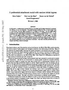
(a) Intake distribution

(b) Inter-intake time distribution

Figure 2. Probability plots for the distribution fitting (Adult Female, 15-45). After the work of [57], the intake distribution FU is modeled by a heavy-tailed distribution, namely the Burr distribution (of which cumulative distribution function is of the form (1 − (1 + xc )−k ), with c > 0 and k > 0). It is noteworthy that it fulfills assumption H3 (see Remark 3). It is fitted here by means of standard maximum likelihood techniques (see Fig. 2(a) below for a probability plot illustrating the goodness of the fit).

50

´ ´ PATRICE BERTAIL, STEPHAN CLEMENC ¸ ON, AND JESSICA TRESSOU

The times of consumption available from the INCA survey allow us to compute the inter-intake times or at least produce right censored values (providing then the information that some durations between successive intakes are larger than a certain time). A Gamma distribution (which has increasing hazard rate) is retained for modeling the inter-intake distribution G: its parameters are fitted using a right censored maximum likelihood procedure. As shown by the probability plot displayed in Fig. 2(b), the chosen distribution (Gamma) provides a good fit for the left (uncensored) part of the distribution. The pharmacokinetics of MeHg has been thoroughly investigated in several studies (see [49], [55], [56], and [35] for instance), almost all coming to the conclusion that the half-life of methyl mercury in man (see Remark 1) fluctuates around six weeks. As we could not dispose of any raw data related to MeHg half-life in the human body, based on the most documented study (in which collected half-life data (in days) are indicated to range from 36 to 65 and correspond to a sample mean of 44, refer to [56] and [35]), a Gamma distribution with mean 44 days and 5th percentile 36 days is chosen here for modeling the variability of the biological half-life log 2/θ. Table 1 sums up the characteristics of the three input distributions, with the convention that a Gamma distribution with parameter α and β has density given by Γ(α)−1 β −α xα−1 exp(−x/β), and mean αβ. Recall that the tail index of the Burr distribution is given by κ = (ck)−1 and its moment of order r is finite if ck > r, it is then given by Γ(k − r/c) × Γ(1 + r/c)/Γ(k). Table 1. Parameters of the input distributions (Adult Female, 15-45; fitted by maximum likelihood). Intake distribution Sample size Burr Parameters Tail index Mean Intake Inter-intake time distribution Sample size Proportion of censored data Gamma Parameters Mean inter-intake time Half-Life distribution Gamma Parameters Mean half-life

FU n c k κ mFU G n α β mG α β

(Unit: µg/kgbw/meal) 1088 0.95 4.93 0.214 0.243 (Unit: hour) 1214 47.4% 1.07 117.21 125 (Unit: hour) 13.6 77.4 44 × 24

Time to steady-state. As underlined in Remark 5, the question of determining how much time is needed for the exposure process to be roughly at equilibrium is crucial for assessing the practical relevance of steady-state characteristics. In order to evaluate the time to steady-state, Monte-Carlo simulations have been carried out: using the instrumental distributions described above, M = 1000 trajectories

A STORAGE MODEL FOR MODELING EXPOSURE TO FOOD CONTAMINANTS

51

have been started from different initial values x0 . For each path, the (temporal) mean exposure over the time interval [0, T ] is computed and individual results have been averaged. In Figure 3(a), the resulting estimates for the Adult Female (1545) subpopulation are displayed, as time T grows: as expected, all empirical mean exposures converge to the same quantity (namely mµ ) and the relative error is lower than 10% after 29 half-lives (3.5 years approximately), whatever the starting value x0 . The same procedure is used for the mean time spent beyond the reference threshold u = Xref,0.7 : as shown by Figure 3(b), the limit is approximately reached after 70 half-lives (about 8.5 years), whatever the initial state x0 . The convergence is slower in this case, since the quantity of interest is related to an event of relatively small probability (see also Remark 10). Naturally, the time to steady-state strongly depends on the initial value x0 and of the functional of interest. However, on the basis of these simulation results, it may be stated that, for realistic initial values, the time to steady-state for basic quantities as the ones considered here fluctuates between 3 and 10 years, which is a reasonable horizon at the human scale.

(a) Mean exposure versus time

(b) Average time spent over u versus time (u = Xref,0.7 = 6.42 µg/kgbw)

Figure 3. Convergence to steady-state (Adult Female, 15-45; x0 = 0, 1.2, 2.4, 3.6, 4.8, 6). Remark 8. (Convergence rate bounds) The problem of determining computable bounds on the convergence rate of ergodic Markov processes has recently received much attention in the applied probability literature (see [42], [53], [39], [51] or [52]). Using suitably calibrated parameters of the drift and minorization conditions (Equations (18), (19), (23), and (22)) established along the proofs of theorems 3.1 and 3.2 in the Appendix, rough numerical estimates of the constants involved in rate bounds (10) and (12) can be computed from Theorem 2.2 in [52] (in the discrete-time case) and Theorem 4.1 in [52] (in the continuous-time setup). Explicit computations based on these theoretical results shall be carried out in a forthcoming paper (see [7]). However, as such computable bounds are quite loose in general and are related to the total variation norm (whereas one rather focuses on specific functional of interest in practice), the problem is handled here by exploiting the simulation approach.

52

´ ´ PATRICE BERTAIL, STEPHAN CLEMENC ¸ ON, AND JESSICA TRESSOU

Estimation by computer simulation. We now focus on estimating certain relevant time-dependent and steady-state quantities among those enumerated in the previous section via the simulation approach studied in Section 4 from our MeHg datasets. Estimates of the quantities of interest are computed by averaging over M = 1000 replicated trajectories on [0, T ], taking T equal to 5 years. In order to ensure that the retained trajectories are approximately stationary, a burn-in period of 5 years is used (see the preceding paragraph). Numerical results related to the estimation of the steady-state mean exposure (mµ ), the probability to exceed the dynamic reference doses in steady-state (µ([Xref,0.7 , ∞[) and µ([Xref,1.6 , ∞[), the mean time to run over the lowest reference dose (Eµ [τXref,0.7 ]) and the expected maximum exposure over 5 and 10 years (Eµ [maxt≤5/10 years X(t)]) are displayed in Table 2. Table 2. Estimated features of the exposure process (Adult Female, 15-45). Parameter Unit mµ (µg/kgbw) µ([Xref, 0.7 , ∞[) (%) µ([Xref, 1.6 , ∞[) (%) Eµ [maxt≤5 years X(t)] (µg/kgbw) Eµ [maxt≤5 years X(t)] (µg/kgbw)

Estimate 2.92 0.575 0.003 6.63 7.41

We observe that the average time spent over the EU-based threshold (Xref,1.6 ) or the US-based one (Xref,0.7 ) are close to zero in the Adult Female (15-45) subpopulation, resp. 0.003% and 0.575%. Regarding the time required to reach such threshold levels, further simulations have been conducted using the estimated stationary mean as the initial point (namely, x0 = 2.92). Only the distribution of the time to reach the US-based threshold (Xref,0.7 ) has been estimated using a standard Monte-Carlo procedure As explained in Remark 10 below, estimating the distribution of the time required to run over level Xref,1.6 involves computing rare event probabilities and thus requires the use of more sophisticated simulation meth+ ods. Over M = 1000 trajectories, the mean (respectively, the median) of τX ref,0.7 is 7.23 years (resp. 5.05 years). Figure 4 displays the (highly skewed) Monte-Carlo distribution estimate (obtained by a kernel estimation built over the M = 1000 simulated values using a standard procedure) of the time to run beyond Xref,0.7 for the studied subpopulation. Remark 9. (Sensitivity to the instrumental distributions) The distribution models used here for the governing probability measures FU and G have been chosen because they provide a good overall fit to the data (and may be easily seen to satisfy all the assumptions required in the ergodicity and stability analyses). According to our own practical experience, the numerical results displayed here would not have been significantly different, if one had chosen to model G by a Weibull distribution for instance. However, in a future study (see [7]) special attention shall be given to the statistical issues of validating the mathematical toxicological model, by investigating how sensitive the latter is to changes with respect to the estimation method chosen (considering also the use of nonparametric approaches).

A STORAGE MODEL FOR MODELING EXPOSURE TO FOOD CONTAMINANTS

53

Figure 4. Monte-Carlo distribution for the time to run over u for the Adult Female (15-45) subpopulation (u = Xref,0.7 = 6.42 µg/kgbw, with x0 = 2.92). Remark 10. (Naive Monte-Carlo simulation and high threshold) From the perspective of public health guidance practice, it is of prime importance to evaluate the probability of occurrence of rare (extremely risky) events, the probability to exceed a large threshold u such as u = Xref,1.6 for instance. In this respect, we point out that the naive Monte-Carlo simulation proposed here leads to estimate this probability by zero (see Table 2), so seldom this threshold is reached on a time interval [0, T ] of reasonable length. Treading in the steps of [16], it is shown in [7] that one may remedy to this problem by implementing a suitable particle filtering algorithm. Appendix A. Technical proofs. A.1. Proof of Theorem 3.1. From conditions required by Theorem 2.1, aperiodicity and irreducibility properties are immediately established for the discrete-time ˜ In addition, under mild irreducibility conditions, the stability of the chain X. random coefficients autoregressive model on Rd Yn+1 = αn Yn + βn , where (αn , βn ), n = 1, . . . are i.i.d. r.v.’s on R∗+ ×Rd , has been investigated in detail since the seminal contribution of [37] (see [48] and the references therein). Under the assumption that E[log(1 ∨ kβ1 k)] < ∞ and E[log(1 ∨ α1 )] < ∞, it is well known that a sufficient and necessary condition for the chain X to have a (unique) probability measure is that E[log(α1 )] < 0 (see Corollary 2.7 in [11] for instance). Based on this result, it is then straightforward that, under the assumptions of Theorem 2.1 ˜ is positive recurrent with absolutely continuous stationary and (H1), the chain X probability distribution µ ˜(dx) = f˜(x)dx. In the discrete-time context, analysis of the stability of Markov models (Yn )n∈N may be carried out by establishing suitable conditions for the ’drift’ ∆V (y) = E[V (Y1 ) | Y0 = y] − V (y) for appropriate non-negative test functions V (y). Such ’FosterLyapunov’ criteria stipulate the existence of a ’small set’ S (i.e., an accessible set S to which the chain returns in a given number of steps with positive probability,

´ ´ PATRICE BERTAIL, STEPHAN CLEMENC ¸ ON, AND JESSICA TRESSOU

54

uniformly bounded by below, see section 5.2 in [44]) toward which the chain drifts in the sense that: ∆V (x) ≤ −f (x) + bI{x∈S} , (18) ˜ any for some ’norm-like’ function f (x) ≥ 1 and b < ∞. Now for the chain X, compact interval [0, s] with s > 0 is small. Indeed, it follows from (9) that for all x ∈ [0, s], the minorization condition below holds: Π(x, .) ≥ δs · Us (.),

(19)

with δs = s × inf y∈[0,s] fU (y) > 0 and denoting by Us (.) the uniform probability distribution on [0, s]. When γ = 1 for instance, take V (x) = 1 + x. The affine drift ˜ is given by related to X ∆V (x) = −cx + E[U1 ], with c = 1 − E[e−θ1 ∆T2 ] > 0. Choosing S = [0, s] with s ≥ 1 + 2E[U1 /c], (18) is fulfilled with f (x) = cV (x)/2 and b = E[U1 ] + c/2. Applying Theorem 15.0.1 in ˜ is geometrically ergodic with invariant probability measure [44], we thus get that RX ∞ µ ˜ such that µ ˜(V ) = x=0 V (x)˜ µ(dx) < ∞. In particular, µ ˜ has finite expectation and there exist constants r > 1, R < ∞ such that for all x > 0: ∞ X

rn kΠn (x, .) − µ ˜kV ≤ RV (x),

(20)

n=0

R with kνkV = supψ:|ψ|≤V ψ(x)ν(dx) for all bounded measure ν on the real line. When V ≡ 1, k.kV coincides with the total variation norm k.kT V . For γ > 1, the results is proved in a similar fashion by taking V (x) = 1 + xγ . Finally, the last assertion of Theorem 3.1 immediately derives from Theorem 1 in [32]. A.2. Proof of Theorem 3.2. Set X0 = X(0). Observe that for all t > 0, X(t) = XN (t) e−θN (t) A(t) , so that X(t) ≤ XN (t) . Hence, we naturally have {X(t) → ∞} ⊂ ˜ is positive recurrent with {Xn → ∞}. Therefore, under (H1), we know that X stationary distribution µ ˜, so that in particular P(Xn → ∞) = 0. Furthermore, observe that for all t > 0, u ≥ 0: Z

t

I{X(s)≥u} ds = s=0

Therefore, for all k ∈ N,

N (t) Z Tk X k=1

R Tk+1 s=Tk

s=Tk−1

Z

t

I{X(s)≥u} ds +

I{X(s)≥u} ds. s=TN (t)

I{X(s)≥u} ds = I{Xk ≥u} · ∆Tk+1 ∧

log(Xk /u) . θk

Now, applying the strong law of large number (SLLN) to the positive recurrent chain ((Xn , θn , ∆Tn+1 ))n∈N with invariant probability distribution µ ˜(dx)⊗H(dθ)⊗ G(dt), we get that Z ∞ Z Z ∞ n Z Tk+1 X log(x/u) −1 n I{X(s)≥u} ds → t∧ µ ˜(dx)H(dθ)G(dt). (21) θ s=Tk x=u θ∈Θ t=0 k=1

As we assumed mG = E(∆Tk ) < ∞ for k ≥ 2, we have the following convergence for the delayed renewal process: N (t)/t → m−1 G as t → ∞. Combined with (21), Rt this yields t−1 s=0 I{X(s)≥u} ds → µ([u, ∞[) as t → ∞, with µ given by (11).

A STORAGE MODEL FOR MODELING EXPOSURE TO FOOD CONTAMINANTS

55

We thus proved that X(t) has a limiting probability distribution µ, which has density f (y) given by Z Z ∞ −1 ¯ f (y) = mG f˜(yeθt )eθt G(t)dtH(dθ), θ∈Θ

t=0

¯ = 1 − G the inter-intake survival function. denoting by G Besides, if sup Θ < ∞, from (11), we immediately have that, for all u > 0, t > 0, t ∧ log 2 ¯ G(t)˜ µ([2u, ∞[) ≤ µ([u, ∞[) ≤ µ ˜([u, ∞[). mG sup Θ The distributions µ and µ ˜ have thus exactly the same right tail behavior. Assuming now that (H2) and (H4) are both fulfilled, we turn to the study of the trivariate process {(X(t), θ(t), A(t))}t≥0 . It may be easily seen as λ ⊗ H ⊗ G¯ irreducible and any compact set [0, s]×[0, θ]×[0, a], with s > 0, θ¯ > 0, a > 0 is a ’petite set’ for the latter (see [43] for an account of stochastic stability concepts related to continuous-time Markov processes). Indeed, denote by Qt (. | (x0 , θ0 , a0 )) the distribution of (X(t), θ(t), A(t)) conditioned upon (X(0), θ(0), A(0)) = (x0 , θ0 , a0 ). One may easily check that its trace on the event {N (t) = 1} has density fU (eθa x − ¯ x0 e−θ0 (t−a) )eθa G(a)g a0 (t − a) with respect to λ(dx) ⊗ H(dθ) ⊗ λ(da). Hence, for ¯ × [0, a], we have the minorization condition: all (x0 , θ0 , a0 ) ∈ [0, s] × [0, θ] ¯ a) · Us ⊗ H(. ∩ [0, θ]) ¯ ⊗ Ua , Qt (. | (x0 , θ0 , a0 )) ≥ δ(s, θ,

(22)

¯ a) = (s × H([0, θ]) ¯ × a) · inf ¯ ¯ with δ(s, θ, x∈[0,seθa ] fU (x) · inf v∈[t−a,t] ·g(v)G(a). Following [38] (see Theorem 4.1 therein), let η, δ be such that 0 < η < δ and consider the Lyapounov V (x, θ,i t) = (1 + xγ )(1 + θ)W (t) on R3+ with h function R ∞ dx (notice that, under (H4), W (t) → ∞ as W (t) = 1 + G(t)e−ηt 1 + x=t eδx G(x) G(t) t → ∞). It may be easily seen that the test function V belongs to the domain of the infinitesimal generator G (see Eq. (5)) and that GV (x, θ, t) = −ηV (x, θ, t) + b(x, θ, t), where b(x, θ, t)

(1 + xγ ) (1 + θ) [z(t) − θγxγ W (t)]

=

− ζ(t) [(1 + xγ )(1 + θ) − (1 + E [θ]) (1 + E [(x + U )γ ])] ,   Z ∞ g(t) −ηt δu ¯ 1 − 2G(t) + e G(u)du − G(t)e(δ−η)t . z(t) = η + ¯ e G(t) u=t Observe that b(x, θ, t) → −∞ as (x, θ, t) tends to infinity. Hence, there exist s > 0, θ¯ > 0 and a > 0 large enough and b < ∞ such that the following drift condition holds: GV (x, θ, t) ≤ −ηV (x, θ, t) + bI{(x,θ,t)∈[0,s]×[0,θ]×[0,a]} . ¯

(23)

Then, (12) directly follows from Theorem 5.3 in [41]. A.3. Proof of Proposition 1. Given (X(0), A(0)) = (x0 , a), we have for all T > 0, ¯ T = T −1 X

Z

T1

t=0

X(t)dt + T −1

N (T )−1 Z Tk+1 X k=1

t=Tk

X(t)dt + T −1

Z

T

X(t)dt. TN (T )

(24)

´ ´ PATRICE BERTAIL, STEPHAN CLEMENC ¸ ON, AND JESSICA TRESSOU

56

The first term on the right-hand side of (24) being bounded by x0 T1 /T , it almost surely converges to 0 as T → ∞. Also, we have for all k ≥ 1, Z Tk+1 Xk X(t)dt = (1 − e−θk ∆Tk+1 ). θk t=Tk Furthermore, by virtue of Theorem 3.1, assumption (H2) with γ = 1 ensures that R∞ mµ˜ = x=0 x˜ µ(dx) < ∞ and consequently that Z ∞ Z ∞Z x(1 − e−θt ) m ˜ = µ ˜(dx)H(dθ)G(dt) < ∞, θ x=0 t=0 θ∈Θ making P the SLLN for the positive recurrent chain ((Xn , θn , ∆Tn+1 ))n≥1 applicable to n≥1 (1 − exp(θn ∆Tn+1 ))Xn /θn (refer to Theorem 17.3.2 in [44] for instance). We thus have that

N

−1

N X Xk k=1

θk

(1 − e

−θk ∆Tk+1

Z

∞

Z

) → mµ˜ t=0

θ∈Θ

1 − e−θt H(dθ)G(dt) a.s., θ

(25)

as N → ∞. Combining (25) with N (T )/T → m−1 G a.s. as T → ∞, this entails that the third term in (24) tends to 0 as T → ∞ and establishes (13). Notice that R∞ R mµ = t=0 θ∈Θ (1 − exp(−θt))/θH(dθ)G(dt)mµ˜ /mG . We now turn to the proof R of the Central Limit Theorem (CLT). Using again Theorem 3.1, we have that x2 µ ˜(dx) < ∞ when (H2) holds for some γ ≥ 2, so that Z ∞ Z ∞Z x2 (1 − e−θt )2 µ ˜(dx)H(dθ)G(dt) < ∞. θ2 x=0 t=0 θ∈Θ By virtue of the CLT for positive recurrent chains (see Theorem 17.0.1 in [44]), PN we have that N −1/2 k=1 {(1 − e−θk ∆Tk+1 )Xk /θk − m} ˜ converges in distribution to −θ1 ∆T2 P∞ X1 (1−e−θ1 ∆T2 ) ) 2 2 −m) ˜ 2 ]+2 k=2 Eµ [( X1 (1−eθ1 − N (0, σ ˜ ) as N → ∞, with σ ˜ = Eµ [( θ1 −θk ∆Tk+1

m)( ˜ Xk (1−e θk

)

− m)]. ˜

One may then easily deduce (14) from (24) with σ 2 = σ ˜ 2 /mG . A.4. Proof of Theorem 4.1. Observe first that (16) immediately follows from (15) by virtue of standard properties of Wasserstein metrics. In order to prove (15), we construct a specific coupling of the laws LXˆ (T ) and LX (T ) . Let (Vk )n∈N , (Vk0 )k∈N and (Vk00 )k∈N be three independent sequences of i.i.d. r.v.’s, uniformly distributed on [0, 1]. For all (n, k) ∈ N2 , set ∆Tk = G−1 (Vk ), Uk = FU−1 (Vk0 ), θk = H −1 (Vk00 ), (n)

∆Tˆk

−1

(n)

ˆ (n) (Vk ), U ˆ =G k

(n)−1

= FˆU

(n)

(Vk0 ), θˆk

−1

ˆ (n) (Vk00 ), =H

ˆ (n) = and define recursively for k ∈ N, Xk+1 = Xk e−θk ∆Tk+1 + Uk+1 and X k+1 (n) (n) ˆ (n) e−θˆk ∆Tˆk+1 + U ˆ (n) with X0 = X ˆ (n) = x0 , as well as Tk+1 = ∆Tk+1 + Tk X 0 k k+1 (n) (n) (n) (n) and Tˆk+1 = ∆Tˆk+1 + Tˆk with T0 = Tˆ0 = 0. For notational convenience, the superscript (n) is omitted in the sequel. Using in particular the fact that x ≥ 0 7→ e−x

A STORAGE MODEL FOR MODELING EXPOSURE TO FOOD CONTAMINANTS

57

is 1-Lipschitz, straightforward computations yield k k X X ˆ ∆Tˆi+1 θi − θˆi } θi ∆Ti+1 − ∆Tˆi+1 + Xk − Xk ≤ x0 { i=1

i=1

+

k X

k−1 X

Ui (

i=1

k k−1 X ˆ X ˆ ∆Tj+1 θj − θˆj ) + θj ∆Tj+1 − ∆Tˆj+1 + Ui − Ui

j=i

i=1

j=i

(26) Turning now to the coupling construction in continuous time, define N (t) = P ˆ k≥1 I{Tk ≤t} and N (t) = k≥1 I{Tbk ≤t} , as well as X(t) = XN (t) exp(−θN (t) (t − ˆ ˆ TN (t) )) and X(t) = XNˆ (t) exp(−θˆNˆ (t) (t − TˆNˆ (t) )) for t ≥ 0. Set also Tk+ = Tk ∨ Tˆk and T − = Tk ∧ Tˆk for all k ∈ N and observe that

P

k

mH (ΓXˆ (T ) , ΓX (T ) ) ≤

max

ˆ (T ) 0≤k≤N (T )∨N

Mk ,

(27)

where Mk =

sup − Tk+ ≤t