more than 40 Msamples/s when processing 3-dimensional streaming data and up to 1.78 Msamples/s for 70-dimensional data.
A Streaming Clustering Approach Using a Heterogeneous System for Big Data Analysis Dajung Lee* , Alric Althoff+ , Dustin Richmond+ , Ryan Kastner+ The Department of Electrical and Computer Engineering* The Department of Computer Science and Engineering+ University of California, San Diego La Jolla, CA, USA {dal064, aalthoff, drichmond, kastner}@eng.ucsd.edu
Abstract—Data clustering is a fundamental challenge in data analytics. It is the main task in exploratory data mining and a core technique in machine learning. As the volume, variety, velocity, and variability of data grows, we need more efficient data analysis methods that can scale towards increasingly large and high dimensional data sets. We develop a streaming clustering algorithm that is highly amenable to hardware acceleration. Our algorithm eliminates the need to store the data objects, which removes limits on the size of the data that we can analyze. Our algorithm is highly parameterizable, which allows it to fit to the characteristics of the data set, and scale towards the available hardware resources. Our streaming hardware core can handle more than 40 Msamples/s when processing 3-dimensional streaming data and up to 1.78 Msamples/s for 70-dimensional data. To validate the accuracy and performance of our algorithms we compare it with several common clustering techniques on several different applications. The experimental result shows that it outperforms other prior hardware accelerated clustering systems. Index Terms—Online clustering, streaming architecture, hardwaresoftware codesign, FPGA, hardware acceleration, vector quantization
I. I NTRODUCTION Data clustering is one of the fundamental problems in data analytics, pattern recognition, data compression, image analysis, and machine learning [1]–[4]. Its goal is to group data objects that most resemble one another into the same cluster based upon some metric of similarity, or equivalently to separate data items that are relatively distinct into separate clusters. Clustering algorithms can exhibit vastly different performance depending on the application, thus one must employ the algorithm that best matches the characteristics of the data set. For example, k-means is one of the oldest and simplest clustering algorithm. It partitions input observations into k groups, each of which is represented by a single mean point of the cluster. It is frequently used, likely due to its simplicity, but its basic assumption limits the separability of the data. Furthermore, it uses an iterative approach that does not scale well. There are many variations of the k-means algorithm e.g., [5], [6], and other algorithmic approaches, such as BIRCH or DBSCAN [7], [8] developed to provide better performance or work with datasets with different properties. Increasing amounts of data are created in our daily life. These “big data” sets can be large, high-dimensional, diverse, variable, and delivered at high rates. More importantly, they are commonly time sensitive. The data must be analyzed quickly to extract actionable knowledge. In order to improve our ability to extract knowledge and insight from such complex and large data sets, we must develop efficient and scalable techniques to analyze these massive data sets being delivered at high rates. Online data clustering algorithms handle unbounded streaming data without using a significant amount of storage. Thus, they provide a fast technique that maps well to hardware. However, online clustering has its drawbacks. Generally online algorithms look at the data only
once. While this limits the storage, and thus allows for scalability and more efficient hardware implementations, it can reduce the accuracy compared to other iterative approaches that perform multiple passes over the data. For example, if the data characteristics evolve over time, the online algorithms can get stuck in a local optimum. These issues make it non-trivial to perform an accurate clustering using online algorithms. Yet these algorithms have good scalability and map efficiently into hardware. We propose a multilevel, online data clustering method that is accurate while providing a scalable hardware architecture that is suitable for implementation in a heterogenous systems. Our method approximates multiple subclusters from streaming data first, then applies a problem specific clustering algorithm to these subclusters. Each subcluster is represented using a set of centroids which are estimated with different parameters independently. Each subcluster module accepts streaming input data and keeps updating the centroids set based upon the new data object. The next step to cluster these approximated points maps centroids to clusters, which is determined by the dataset properties. In our method, one cluster can have more than one center points unlike the k-means algorithm which has a single representative point per one cluster. We carefully profile the algorithm and partition the workload across hardware and software. The subclustering process handles a massive amount of data and is a very demanding operation. Therefore we optimize its hardware implementation to perform a onepass process while minimizing computation and space complexity. The next module deals with a relatively small set of data, so it can be processed either in software or hardware depending on a system goals. Our final hardware design achieves high throughput performance with reasonable resource utilization, which enables it to scale towards large and high dimensional data sets. Our clustering method outperforms the state of the art clustering algorithms in software system [5] and FPGA implementations of heterogeneous systems [9]–[11]. The primary contributions of this research are: • A hardware friendly, multilevel, streaming clustering algorithm that can handle large, high dimensional data sets. • A hardware/software codesign method for streaming clustering architecture that achieves high throughput and low resource utilization across a wide set of algorithmic and system parameters • Characterizing our system performance on a wide range of applications including image segmentation and big data analysis of real world datasets The remainder of the paper is organized as follows. Section II describes related work. Section III introduces our streaming data clustering algorithm. We explain our hardware design and optimization methods in Section IV, and show our experimental results in Section V. We conclude in Section VI.
II. R ELATED W ORK There are many clustering algorithm that target different data set properties. Generally it is up to the user to choose the “best” algorithm. Clustering algorithms can be largely divided into several groups, and, in this paper, we consider three popular clustering groups: partitioning, hierarchical, and density-based. We will focus on three algorithms – one from each group (k-means, BIRCH, and DBSCAN). And we specifically compare our work to existing hardware accelerated approaches. k-means is the most used partitioning method, which is commonly known as Lloyd’s algorithm. It finds a set of centroids that represents data clusters. It is the simplest method that is frequently used in practical applications. There exist many variation of k-means algorithm, such as k-median, k-medoids, or k-means++. However, its inherent iterative solution for an optimal centroid set is highly compute and data intensive. As such, there have been many efforts to improve its computing performance [5], [6]. Hierarchical approaches build a hierarchy of clusters based on their similarity, and split down or merge up close clusters. The BIRCH algorithm is a well-known hierarchical algorithm [7]. It minimizes the number of processing passes and is capable of handling large datasets in a limited memory. DBSCAN algorithm is a density-based clustering method [8]. It scans dataset iteratively and finds a data group packed in high density. It can cluster an arbitrarily density shape dataset and has a notion of noise, which makes it robust to outliers. Each algorithm has limitations. The quality of k-means is highly dependent on the initial seed, and it is limited to clusters separable by d-dimensional spherical densities. Its objective function is sensitive to outliers, and its iterative operation makes it hard to scale. BIRCH uses a two-pass process to reduce these issues, but it is sensitive to parameters. And it uses a CF-tree data structure which is difficult to implement efficiently in hardware. DBSCAN is also very sensitive to parameters in terms of accuracy. This algorithm requires iterative operation and needs data to stay in a memory, which makes hard to map to hardware. There are several projects aimed to accelerate clustering algorithms using a custom hardware or heterogeneous system. Hussain et al. [12], [13] accelerate k-means on an FPGA to perform gene analysis. They compare their FPGA implementation with a GPU implementation, and demonstrate speedup and improved energy efficiency on the FPGA. However, the on-chip memory capacity limits the size of data set to a small number of dimensions and a small number of centroids. Lin et al. [9] present a k-means hardware accelerator that uses a triangle inequality to reduce the computational complexity. The accelerator can handle 1024-dimensional data from an external DDR memory, but can only handle a small number (1024) of data points. More recently, Abdelrahman et al. [11] explores k-means on a shared memory processor-FPGA system. They partition the k-means workload across CPU and FPGA. They achieve 2.9× speed up against CPU only implementation and 1.9× faster than an accelerator alone design. However, their work does not support high dimensional data clustering and presents limited results for small numbers of clusters. Some approaches merge hardware acceleration and data structure optimizations. Chen et al. [14] implements a hierarchical binary tree on an FPGA. The tree is generated by splitting the data set recursively. Similarly, Winterstein et al. [10] use a kd-tree and with on-chip dynamic memory allocation in an attempt to efficiently use memory resources. While the accelerator traverses the tree, it updates a set of centroids. This process reduces the computational load, however, their design requires preprocessing to build a tree, and it does not
c1 .
c0 .
. .
. . . c|L|-3 . . . .c . . |L|-2 . c|L|-1
. . . c2 . . . c 3
Subcluster1
Subcluster2
Cluster 0
Subcluster3
.. . .. ... .
..
Centroids generated from subclustering
. ..
.. ...
. .. .
..
L
V
c0
0
c1
0
c2
1
…
…
c|L|-3 0
Cluster 1
c|L|-2 1 c|L|-1 1
Fig. 1. Our multilevel clustering algorithm in two stages. The first stage clusters the same set of data multiple times (three subcluster modules in this example) similar to k-means. It generates |L| = l centroids representing l subclusters that is more than target clusters. Then, it clusters them using an existing clustering algorithm to find a look up table, L × V that maps L centroids to the target clusters V . Data points in subcluster c0 are clustered to cluster 0.
handle a high dimensional data. In general, larger trees do not fit on an on-chip FPGA memory, and traversing the tree requires frequent irregular data accesses that limit performance. Our solution does not have these limitations. As a demand for clustering big data analysis increases, streaming clustering algorithms have gotten more attention as they are more easily scaled to larger data sets. StreamKM++ [5] uses a non-uniformly adaptive sampling approach for k-means to handle streaming data. It uses a coreset tree data structure to bound the data set size while streaming in data. Ailon et al. [6] suggests a streaming approximation of k-means by expanding k-means clusteing algorithm in hierarchical manner. These streaming methods provide a good approximation of k-means and improves its performance by minimizing memory accesses. However, these methods still have significant computational complexity, which hinders their efficiency when mapped to hardware. For example, the coreset tree data structure used in StreamKM++ is hard to implemented in hardware. And the approximation algorithm in [6] still has interation within its process. Our method approximates input data into centroids more efficiently in a streaming way. We use vector quantization [15] to build a streaming clustering architecture on an FPGA. The approximation algorithm minimizes the computation and space complexity, which yields higher performance with less memory space needed. Our architecture is described in more detail the next section. III. S TREAMING C LUSTERING In this section, we introduce our streaming clustering algorithm that handles an unlimited amount of data while achieving high accuracy and suitable for a wide range of applications. A. Multilevel clustering Our clustering method sets multiple representations for each cluster (see in Fig. 1). The algorithm is divided into two main stages. We call the first stage subclustering. In this stage, n input data are clustered into l subclusters (k < l < n) in a similar manner to the k-means algorithm. In the second stage, some of these centroids are grouped together into a larger cluster. We call this reduction stage. Each subcluster is generated from the same set of input data, but use different parameters.
Current center
Algorithm 1: Streaming subclustering (x,C) Input : x is a streaming input in d dimension, C is a current set of centroids Output: C is the latest set of centroids
New point coming Data points New center
At time t
1
At time t+1
2
Fig. 2. When a new data point comes in, a center point that locates close moves toward the new point. This process keeps updating and moving around this center point as a new data appears.
3 4 5
Accept a new input x Calculate distance between each center point c ∈ C and the current input x Get a center point of the nearest cluster, cm . Move cm closer to x Return the current C
For example, three subcluster modules in Fig. 1 consider the same data and generate k center points from each. These center points sets compose the l centroids. These l centroids, L = {c0 , c1 , ..., cl−2 , cl−1 }, are clustered in reduction stage using a problem specific clustering algorithm. Clustering algorithms are sometimes very sensitive on choosing right parameters or initial seeding points. Our method can reduce the dependency on a particular parameter by using these different subclustering results. The final result is a single lookup table that maps a set of centroids, {c0 , c1 , ..., cl−2 , cl−1 }, and corresponding cluster ID, {0, 1}. We have the final result clustered 0 or 1 either. For example, based on this look up table, all data having c0 for the nearest centroid are assigned cluster 0, and other data closer to c2 are clustered to cluster 1.
The step size for this update is decided by the current input, the center point, and a learning rate, α. The learning rate is a weight of the current input data where xt is a current input at time t, cmt is a clustered center point for xt−1 , and cmt+1 is an updated center point. The initial seeding problem is an important issue for clustering algorithms, such as k-means or vector quantization, to find a global optimum. k-means++ defines the precondition problem in k-means and suggests a solution for better accuracy. In other works, initial centroids are randomly chosen in general. Our method accepts an unbounded input stream, so we can feed subclustering modules a random points or use a precalculated set from software side with a small subset of data in first part of data sequence using k-means.
B. Streaming Subclustering
C. Reducing
Subclustering and reduction are key operations in our method. Subclustering stage processes a large size input data and generates centroids. Reducing handles a smaller set of approximated centroids. Subclustering is very data intensive and computationally demanding process while reduction is much lighter. To minimize overall computation and space complexity for big data analysis, we focus making the subclustering operation into a hardware friendly streaming algorithm. It is based on a streaming version of vector quantization, which is also closely related competitive learning or a leader-follower clustering algorithm [16]. Vector quantization is used for data compression in signal processing. It partitions the data into subsets (clusters), which are modeled as probability density functions represented by a prototype vector (centroid). The simplest version for vector quantization picks data vector randomly from a given dataset. Then, it determines its appropriate centroid, and updates the quantization vector centroid based upon that new data object. This vector moves to the current input points and it continues this process for the entire dataset. These steps can be done in one pass and easily implemented in a hardware architecture. Our subclustering hardware module is built upon this streaming vector quantization technique. We assume that the input data is randomly ordered and stationary. Fig. 2 shows an example of how our subclustering module works. If a new data point appears, the closest center point to the new data moves slightly towards it. It keeps updating and moving around this center point. Algorithm 1 presents the streaming subclustering algorithm. Input x is a d-dimensional streaming data point, and C is a set of current centroids for k clusters. The output is the new set of centroids, C. First, a processing core accepts input data, and it calculates distance from this current input to each centroid of k clusters. This point will be assigned to the closest cluster, and that cluster’s center point is updated to consider the new input using the following equation:
The reducing stage is defined at a high level in (2). Its input is K m S = Ki such that Ki = subclusteri (input) where m is the number of
cmt+1 = (1 − α) · cmt + α · xt
(1)
i=1
subcluster modules; there are three subclusters in Fig. 1, for example. The output is L ×V , a lookup table that maps centroids to assigned cluster IDs. Reduction : K → L ×V
(2)
A reduction stage can use any clustering algorithm depending on applications or dataset properties. In this paper, we demonstrate our system with three clustering methods for this stage: minimum cost pick, DBSCAN, and BIRCH. Minimum cost pick is the simplest method. Each subclustering module calculates a cost, an averaged sum of distances between a centroid and data points within the cluster. It compares cost values from every subclustering modules and chooses a single set that has the minimum cost. In this case, L = Ki and V = {1, 2, ..., |V |} such that i = argmin(costi ). DBSCAN i
and BIRCH algorithms cluster these centroids as input. DBSCAN keeps scanning these points multiple times and finds associated data points within a fixed distance. The distance is defined as a parameter, epsilon, and if a cluster does not have enough number of elements, minpts, it considers the cluster as a noise. In this method, L = K and V = dbscan(K, epsilon, minpts). BIRCH generates a tree structure based on two different distance metrics while scanning input data, called CFtree. Then, it scans the initial CFtree and rebuilds a smaller one, and it applies a clustering algorithm to all the tree leaf entries. For BIRCH algorithm, L = K and V = birch(K,threshold). D. Shuffling data Our streaming subclustering module runs based on an assumption that the order of incoming data is random and stationary. However, it does not necessarily hold for all applications. Therefore we add the ability to randomize the dataset. In a streaming process, the processor does not have a control over input sequence coming that is
Software
A. Heterogeneous system
Hardware
input
< software latency > FIFO
Shuffling Streaming subclustering Processing centroids
Shuffling
< 5%
Streaming subclustering
> 90%
Reducing
< 7%
Reducing centroids
Fig. 3. Overall system flow of our heterogeneous clustering system. Streaming subclustering is the most computationally intensive function, so it is accelerated in hardware. The Reducing function can be placed in hardware or software.
unbounded. To make this practical, we shuffle a data array within a fixed window. This randomness makes our method more robust and improves accuracy in final results. Randomization also helps the streaming approach better approximate a non-streaming algorithm. For example, k-means keeps revisiting input data until a solution converges into an optimal point. Instead of scanning the entire dataset multiple times, which is expensive in hardware, we divide the input dataset into several windows. The algorithm scans each window only once, which approximates scanning the original data iteratively. We can vary the size of the window. A larger shuffling window provides a result that closer to an offline method though it requires more hardware resources. Our experiment shows a fully sorted dataset results in a higher error, which can be significantly reduced through randomization to provide similar accuracy as k-means. E. Design parameters Data clustering is employed in all kind of different data sets that vary in dimension, the number of clusters, data size, data type, or other attributes. For example, multimedia data commonly has RGB 3-dimensional data, but other data can have significantly more features [17]. Our proposed system accommodates different clustering parameters for various applications. We have several parameters to build a streaming subclustering core on a hardware: dimension d, the number of clusters k, and learning rate α. A streaming system does not have a limitation on data size. So the dimension and the number of clusters mainly determine throughput performance and resource utilization. Therefore, we focus on optimizing a hardware core to handle different dimensions and different numbers of clusters while retaining the maximum throughput. The learning rate α affects the updating centroids operation. We set different subclustering modules to run with different learning rates. Clustering algorithms in reduction stage also has important parameters, e.g. epsilon and minpts for DBSCAN. However, they are highly application-specific and depend on data set properties, so we do not discuss them. We present our experimental results with different design parameters in Section V. IV. S YSTEM I MPLEMENTATION In this section, we describe our CPU-FPGA heterogeneous system design. The input is an unbounded data stream, and output is a lookup table that describes the centroids and clusters.
The overall system flow consists of shuffling, streaming subclustering, and reduction (see in Fig. 3). According to our software profiling results using example datasets, subclustering stage takes almost 90% of total latency on average. Shuffling is less than 5%, and reduction is around 7%. We focus on accelerating the main bottleneck module, streaming subclustering stage, and additionally implement minimum cost pick and DBSCAN methods in reduction stage on an FPGA. Fig. 4 presents an accelerated core on an FPGA. Shuffling is implemented in software because it is not a compute intensive module, and its frequent data accesses limit it’s acceleration capabilities on the FPGA. To communicate between CPU and FPGA, we employ RIFFA framework [18] and connect our FPGA core to RIFFA with the AXIS streaming interface. B. Subclustering module The Subclustering module processes the same input sequence with different parameters multiple times. Each process is totally independent, so they are highly scalable in hardware. Our streaming approach minimizes computation complexity as well as hardware resources and we parallelize these independent operations. Fig. 5 presents the subclustering core. The accelerator core starts by calculating the distance between the current input data object and the centroid for each of the k clusters. We used L1 norm (i.e., Manhattan distance) for our distance metric. This exposes significant instruction level parallelism as the calculation performs an absolute difference operation on the dimension of input data object and elements of the centroid vector, and then sums these differences. More precisely it performs a sum of absolute differences which maps in a very efficient and scalable manner to an FPGA. The distance calculation is done in a fully parallel manner. We perform complete memory partitioning on the centroid points, i.e., they are stored in registers that can all be accessed in one cycle to allow for high bandwidth accesses. The entire core is parametrized. A user defines parameters, d, k, α, and data type of the data objects. A data clustering core is automatically synthesized based upon these parameters. The entire process is fully pipelined. Every time a new input arrives, the core continues processing and generates one output per input. It takes d clock cycles (dimension of the data objects) to accept d data objects. So the optimal pipeline initiation interval (II), i.e., our target performance, is d clock cycles. C. Reducing module We implement the minimum cost pick and DBSCAN methods on an FPGA for the reduction stage. The BIRCH algorithm uses a tree based data structure that is non-trivial to be implemented on hardware, so we leave that in software. Minimum cost pick simply compares cost values from every subclustering modules and chooses the one set that has the minimum cost value. This module is easily implementable in hardware. The DBSCAN algorithm scans the dataset multiple times. This iterative scanning operation causes high latency for a large size datasets and uses many resources. To achieve high performance, it requires intensive hardware optimization. However, since we handle much smaller size data in reduction module than in the subclustering module, it does not need high performance. We utilize an open source code for DBSCAN [19] to synthesize a hardware architecture using a high level synthesis tool. We optimize the code to use a FIFO module to keep the associated candidate data point for a cluster, instead of a linked list data structure originally used in software.
L {K1, cost1}= subcluster1(input)
Subcluster1
K1
{K2, cost2}= subcluster2(input)
Subcluster2
K2
{K3, cost3}= subcluster3(input)
Subcluster3
K3
V
c10 0 c11 0 c12 1
Reduce
…
…
c57 0 K
L V
c58 1
c59 1
Fig. 4. Hardware design for the multilevel streaming clustering. Streaming subclustering modules are fully parallelized since they are independent from each other. Reducing module merges subcluster centroids and finds final cluster ID for each point.
D
Input
TABLE I T EST DATASETS
Subclustering Core
[0]
d0
[1]
d1
… Cluster
…
…
m
[K-2]
dK-2
[K-1]
…
dK-1 Update Copy
Centers [m]
Fig. 5. A processing core for streaming subclustering operation. It accepts d-dimensional inputs, decides on the appropriate cluster, and updates the corresponding centroid.
V. E XPERIMENTAL RESULTS A. Test environment We evaluated our proposed design on a CPU-FPGA heterogeneous system. Our test system has Intel i7 core 4 GHz and 16 GB DDR in software and a Xilinx Virtex 7 FPGA device, XC7VX485T2FFG1761C, in hardware. We built an accelerator core using Xilinx Vivado HLS 2016.4. We integrated the FPGA core with RIFFA [18] to connect to a CPU and used the Vivado 2016.4 to generate a bitstream file. We verify our approach using several different application datasets with different parameters. Table I presents eight example datasets: synthetic datasets of different shapes in 2D and 3D dimensions – blobs, moons, circles, and 3D clouds, datasets from from UCI Machine Learning Repository (spambase and census 1990) [17], and image segmentation examples in biomedical research – cell images in 1D and 9D dimensions [20]. Note that 3D clouds is a same synthetic dataset used in [10], which is open source. The 9-dimensional cell images data is generated by 3×3 convolutional windowing over 1-dimensional frame, and this convolutional segmentation method clusters the image based on its local variance in neighbor. We apply different clustering algorithms in the reduction stage depending on the application. We use DBSCAN for blobs, moons, and circles dataset, BIRCH for image segmentations, and minimum cost pick for 3D clouds and high dimensional real world applications. B. Accuracy We compare our clustering results for the example datasets to other clustering algorithms: k-means, BIRCH, DBSCAN, and streamKM++. Table II presents the clustering results for 2-dimensional synthetic datasets. k-means and streamKM++ methods group data points centered around a single center point for each cluster, so they cannot find true clusters in moons and circles. On the other hand, DBSCAN
data set blobs moons circles 3D clouds spambase census 1990 cell image (1D) cell image (9D)
data size 1,500 1,500 1,500 16,384 4,601 2,458,285 131,072 131,072
dimension (d) 2 2 2 3 57 68 1 9
clusters (k) 3 2 2 128 10 10 10 10
datatype float float float int int, float int int int
is good at clustering these datasets. We choose this algorithm for our reduction process, and it clusters these datasets correctly. TABLE II 2D SYNTHETIC DATA CLUSTERING RESULTS . k- MEANS , BIRCH AND streamKM++ HARDLY FIND RIGHT RESULTS FOR NON - SPHERICAL DENSITY SHAPE DATASETS . O UR METHOD CLUSTERS THEM CORRECTLY. k-means
BIRCH
DBSCAN
StreamKM
Ours
blobs
moons
circles
TABLE III C OMPARISON OF COST RESULTS
3D clouds spambase census 1990
Kmeans 159.85 97.79 37.36
StreamKM++ 158.28 113.92 37.47
Ours 164.21 103.24 37.41
We compare clustering costs – the mean of distances between each centroid and data points in a cluster. The cost value is estimated from an objective function value in (3) as k-means algorithm does. x’s are n input data, {X1 , X2 , ...Xk } present k clusters, and each of them is represented using a single center point, ci . A cost value is available only for minimum cost pick method. Our clustering method shows comparable results to k-means or streamKM++ in Table III. k
argmin X
∑ ∑
i=1 x∈Xi
||x − ci ||L
(3)
TABLE IV C OMPARING SEGMENTATION RESULTS Input
Cell area
Segmentation
(a)
k-means
BIRCH
DBSCAN
StreamKM
Ours
cell image (1D) cell image (9D) (b)
We test our clustering method on image segmentation application. The segmentation results are presented in Table IV. Input image in this application is extremely noisy, and the image contrast is very low. Since the input is blurred in low intensity, it is nontrivial to separate particular pixel area and hard to achieve a good quality of segmentation results. DBSCAN hardly finds cell area since it is oversensitive to parameters. We use BIRCH algorithm in our reduction stage. 1) Data Shuffling: We observe that shuffled data gives a better approximation (close to k-means); the sorted data stream draws centroids off from the optimal locations. Fig. 6 shows how data shuffling process changes the final cost value. 3D clouds data is fully-sorted set with some initial clustering. Without shuffling, its streaming clustering results in a high cost value. We add the data shuffling module and increases the window size gradually. The cost value becomes lower and closer to k-means result. If the dataset is already in random, it does not have much effect on the result, but if it is sorted, then shuffling operation is necessary. Thus sorting can be used depending upon the characteristics of the dataset. cost
3D cloud dataset
210.0
Shuffling+streaming Kmeans Streaming only
37.4 37.2
190.0
37.0
180.0
160.0
Census dataset
37.6
200.0
170.0
cost
Resource utilization increases almost linearly with respect to the data dimension or the number of target clusters. We test our design with a maximum of 70 dimensional data. Targeting 10 clusters, it consumes 50.73% of BRAMs, 0 DSPs, 23.73% FFs, and 44.08% LUTs. To cluster 3-dimensional data into 128 clusters, it consumes 5.05% of BRAMs, 0 DSPs, 20.48% FFs, and 45.08% LUTs. We vary the learning rate at powers of two (e.g., α = 1/8 through 1/64), which is synthesized to a right shift operation; thus the hardware module uses 0 DSPs. If we switch the parameter to an non power of tow, it consumes a few DSPs. Table V compares our FPGA core performance results to other hardware accelerated works for k-means clustering algorithm [9], [10]. Our hardware core is highly optimized for pipelining and provides deterministic performance results decided by the data dimension d. It achieves more than 40 Msamples/s for 3-dimensional streaming data running at 125 MHz. It shows higher FPGA throughput than the results presented in [9], [10]. Considering the result in [10] does not include a latency from preprocessing, our clustering method outperforms their results, and can operate on unlimited size of data. 2) Subclustering Module Analysis: The Subclustering stage is the most computationally intensive and data demanding module in our algorithm. We accelerate this module on an FPGA and evaluate our design with varying parameters: the dimension of data d, and the number of clusters k. It is based on a streaming approach, and performance and resource results do not depend on the dataset size. For the subclustering core analysis, we set a target clock frequency at 250MHz to evaluate its maximum performance. Fig. 7 and Fig. 8 present the throughput and resource utilization results of a single subclustering core with different input data dimension size. We increase the dimension gradually from 1 up to 70. The number of clusters, k, is 16 in this experiment. The target throughput is determined by the input bandwidth, which is presented in Fig. 7. High dimensional data needs more clock cycles to get input point, so input bandwidth is inversely proportional to its dimension. The processing core is able to achieve the target throughput in terms of clock cycles. It can produce output in every input, but the design complexity increases in higher dimensions. It results in running at a lower clock frequency, so the throughput result is less than the performance goal with higher dimensional data. Throughput (Msamples/sec)
1000.00
Processing Unit Input Bandwidth 100.00
36.8 Shuffling+streaming Kmeans Streaming only
36.6 36.4
10.00
36.2
150.0 32 64 128 256 512 1K 2K 4K 8K 16K
32 64 128 256 512 1K 2K 4K 8K
Shuffling window size
Shuffling window size 1.00
Fig. 6. The cost values for different shuffling window sizes. Result becomes closer to k-means result with a larger shuffling window.
C. Performance and Resource Utilization 1) FPGA Core Design: A generated hardware core is fully pipelined and runs in streaming manner. We set our target throughput as input bandwidth, which is determined by the data dimension d and the clock frequency. Each generated architecture can process data at line rate, i.e., one new datum per cycle.
1
2
3
4
5
6
7
8
9
10 20 30 40 50 60 70
Data dimension
Fig. 7. Throughput results by varying the data dimension. Input bandwidth is the maximum throughput that we can achieve, which depends on data dimension.
Fig. 9 presents throughput and resource results by varying the number of clusters k. The data dimension in this experiment is fixed to 3. Ideally, the throughput result is determined by the data dimension, so the throughput result should be same. However, as k grows larger,
TABLE V FPGA CORE PERFORMANCE COMPARISON WITH OTHER FPGA IMPLEMENTATIONS . data size (N)
dimension (D)
Clusters (K)
Lin et al. [9]
1024
1024
10
Winterstein et al. [10]
16384
3
128
Ours
Streaming
3 3 70
10 128 10
8 bit unsigned int 16 bit unsigned int 16 bit unsigned int
Resource uAlizaAon
900
100
Registers (X100)
800
90
BRAMs
700
80 70
600
60
500
50
400
40
300
BRAMs
Registers (Hundreds)
data type
Throughput (Samples/s)
LUTs
10000
200 K
44194
22521
198
-
1.21M