A strongly conservative finite element method for the ... - CiteSeerX

A strongly conservative finite element method for the coupling of Stokes and Darcy flow G. Kanschat∗,1 Department of Mathematics, Texas A&M University, 3368 TAMU, College Station, TX 77843–3368

B. Rivi`ere2 Department of Computational & Applied Mathematics, Rice University, 6100 Main Street, MS-134, Houston, TX 77005–1892

Abstract We consider a model of coupled free and porous media flow governed by Stokes and Darcy equations with the Beavers-Joseph-Saffman interface condition. This model is discretized using divergence conforming finite elements for the velocities in the whole domain. Discontinuous Galerkin techniques are used in the Stokes subdomain and a mixed method is used in the Darcy subdomain. subdomain. This discretization is strongly conservative and we show convergence. Numerical results validate our findings and indicate optimal convergence orders. Key words: Stokes flow, Darcy flow, Beavers-Joseph-Saffman condition, finite element method, mixed finite elements, discontinuous Galerkin, multiphysics 2000 MSC: 35Q35, 65N30, 65N15

1. Introduction The coupling of Stokes and Darcy equations arises from the modeling of groundwater contamination through streams and filtration problems [23, 19]. In this work, a new numerical method is proposed, that employs divergenceconforming velocity spaces, i.e. spaces included in H div (Ω). The Darcy flow is discretized by a mixed finite element method and the Stokes flow by a mixed discontinuous Galerkin (DG) method. The two types of flow are coupled by appropriate interface conditions, namely mass conservation, balance of forces across the interface and the Beavers-Joseph-Saffman’s law [6, 28, 20]. One ∗ Corresponding

author in part by the National Science Foundation through grants no. DMS–0713829 and DMS–0810387 and by the King Abdullah University of Science and Technology (KAUST) through grant no. KUS-C1-016-04 2 Supported in part by the National Science Foundation through grant no. DMS–0810422 1 Supported

Preprint submitted to Elsevier

paper.tex

1808

2009-08-17

15:42:44Z

kanschat

August 17, 2009

advantage of our approach is that exact incompressibility of the velocity is obtained trivially. Another advantage is that the bilinear form only involves one term on the interface. Indeed only the tangential component of the velocity from the Beavers-Joseph-Saffman’s law appears in the scheme. Finally this paper proposes and analyzes a general framework as the scheme is valid for various DG methods, such as the local discontinuous Galerkin and the interior penalty methods. Various numerical methods, such as finite element methods, mixed methods, discontinuous Galerkin methods and combinations of these methods, have been studied in the literature. For instance, finite element methods were studied in [14] and finite element methods coupled with mixed methods have been analyzed in [22]. Primal DG methods using broken Sobolev spaces are analyzed in [25], and they are coupled with mixed methods in [27]. All of these methods exhibit some mass loss depending on the accuracy of the discretization, which is the main reason to propose our new discretization. A conforming mixed method is analyzed in [15]. Stabilized methods are considered in [10, 11, 1]. The plan of the paper is as follows. Section 2 defines the model problem and a corresponding weak formulation. The general scheme is described in Section 3. Its analysis is presented in Section 4. Finally, Section 5 shows numerical examples and conclusions follow. 2. Model problem and weak formulation Let Ω be a bounded polygonal domain in Rd , d = 2, 3. We assume that Ω is divided into two regions ΩS and ΩD , each being a union of polygonal subdomains. Denote by ΓSD the polygonal line that is the interface between ΩS and ΩD . The external boundaries are defined by ΓS = ∂Ω ∩ ∂ΩS ,

ΓD = ∂Ω ∩ ∂ΩD .

In the region ΩS the fluid velocity uS and fluid pressure pS satisfy the Stokes equations: −∇ · (2νD(uS )) + ∇pS = fS ,

in ΩS ,

(1a)

∇ · uS = 0,

in ΩS ,

(1b)

uS = 0,

on ΓS .

(1c)

The deformation tensor is D(uS ) = 12 (∇uS + (∇uS )T ). The coefficient ν > 0 is the fluid viscosity and the function fS is a body force. In the region ΩD the fluid velocity uD and fluid pressure pD satisfy the Darcy equations: ∇ · uD = fD ,

in ΩD ,

(2a)

uD + K∇pD = 0,

in ΩD ,

(2b)

uD · n = 0,

on ΓD .

(2c)

2

paper.tex

1808

2009-08-17

15:42:44Z

kanschat

Here, fD models sinks and sources in the porous medium. The coefficient K > 0 is the permeability of the porous medium. The system of equations is completed by the Beavers-Joseph-Saffman transmissibility conditions at the interface. Let n and τ denote unit normal and tangential vectors to ΓSD , respectively. We assume that n points outward of ΩS . Introducing the phenomenological friction coefficient γ > 0, these conditions read: uS · n = uD · n,

(3a)

pS − 2νD(uS )n · n = pD ,

(3b)

γK −1/2 uS · τ − 2νD(uS )n · τ = 0.

(3c)

We remark that for three-dimensional domains, equation (3c) is satisfied for all tangential vectors to the interface. In order to obtain weak solutions to the set of equations (1)– (3), we introduce the spaces  H div (Ω) = v ∈ L2 (Ω) ∇ · v ∈ L2 (Ω) ,  H0div (Ω) = v ∈ H div (Ω) v · n = 0 on ∂Ω . In the subdomain ΩS , we have to require additionally, that functions are weakly differentiable. Furthermore, if we use the space H0div (Ω), pressure functions will be determined only up to a constant. Thus, the function spaces for our weak formulation will be Z  Q = q ∈ L2 (Ω) q dx = 0 , Ω  div V = v ∈ H0 (Ω) v|ΩS ∈ H 1 (Ωs ) . We also use the standard notation H s (O) for the Sobolev space of order s on a bounded domain O. We use the scalar product notation and norm on Ω, boundaries, faces, and subsets of those, namely Z Z


 u, v Ω = u · v dx, u, v Γ = u · v ds, Ω



u = Ω

Γ

Z

1/2 u2 dx ,



u = Γ

Ω

On V and Q, we introduce the bilinear forms
aD (u, v) = K −1 u, v Ω , D
aS (u, v) = 2ν D(u), D(v) Ω , S

 aI (u, v) = γK −1/2 uS · τ, vS · τ Γ , SD

Z

1/2 u2 ds .

Γ

∀u, v ∈ V, ∀u, v ∈ V, ∀u, v ∈ V,

a(u, v) = aD (u, v) + aI (u, v) + aS (u, v), ∀u, v ∈ V,
b(v, q) = − ∇ · v, q Ω , ∀v ∈ V, ∀q ∈ Q. 3

paper.tex

1808

2009-08-17

15:42:44Z

kanschat

(4)

Throughout the paper, we use the notation vS = v|ΩS . Thus, uS · τ and vS · τ refer to the tangential traces of u and v taken from the side of ΩS at the interface ΓSD . The weak formulation of the problem (1)–(3) reads: find (u, p) ∈ V × Q such that
a(u, v) + b(v, p) = fS , v Ω , ∀v ∈ V,
S (5) ∀q ∈ Q. b(u, q) = fD , q Ω , D

3. Discretization Let Th be a conforming triangulation of Ω such that the interface ΓSD is the union of element edges. For any element T ∈ Th , we denote by hT its diameter and we denote by h the maximum diameter over all mesh elements. Denote by ΓSh the set of edges that are interior to ΩS . Denote by TSh the set of mesh elements that belong to ΩS . As above, we use the scalar product and norm notation on Th , boundaries, faces, and subsets of those, namely X Z X Z


 u, v T = u · v dx, u, v ΓS = u · v ds. h

T ∈Th



u

Th

=

h

T

X Z T ∈Th

1/2 u2 dx ,



u

ΓS h

T

F

F ∈ΓS h

=

1/2 u2 ds .

X Z F ∈ΓS h

F

For the discrete spaces, we use pairs of a divergence-conforming velocity space Vh ⊂ H0div (Ω) and a matching pressure space Qh ⊂ Q, that is of order k. The Stokes operator is discretized by a DG method. In order to do so, we introduce further notation. The jump of traces of a discontinuous function v across interior faces of the mesh is denoted by [[v]]. The following DG norm is used: 





v = ∇v 2 S + σ [[v]] 2 S + h Γ T 1,h h

h

2σ 2 h v ΓS

1/2

,

(6)

where the parameter σ ≥ 0 is the usual penalty parameter of order k 2 . Note that the notation above applies only to quasi-uniform meshes of isotropic cells. On non-uniform meshes, this quantity has to be localized, and on anisotropic cells, the cell size orthogonal to the face should be used and the quotient averaged from both sides. See e.g. [18, 21]. 3.1. Abstract assumptions In what follows, we present an analysis that is valid for various DG methods and finite element spaces. Therefore, we will list conditions on the discretization scheme as a list of assumptions and discuss examples in the following subsection. Assumption 1. ∇ · Vh ⊂ Qh . 4

paper.tex

1808

2009-08-17

15:42:44Z

kanschat

(7)

Our analysis is based on the existence of a projection operator Πh that satisfies several properties. Assumption 2. There exists a projection operator Πh : H0div (Ω) → Vh , satisfying the following properties: 1. Let Ph : Q → Qh be the L2 -projection. The commutation property

q, ∇ · Πh v Ω = Ph q, ∇ · v Ω

(8)

holds for all v ∈ V and q ∈ Q. 2. The value of Πh v on a grid cell K depends on the values of v on K and ∂K only. 3. Πh is stable in L2 (Ω), H div (Ω) and L2 (ΓSD ): there exists a constant Cs independent of hK and h, such that



Πh v ≤ Cs v , (9a) K

K

∇ · Πh v ≤ Cs ∇ · v , (9b)

K

K

(Πh w)S ≤ Cs wS , (9c) ΓSD

ΓSD

for any v ∈ H div (K) and for any w ∈ (H 1 (ΩS ))d . 4. Πh is stable in the DG norm: there exists a constant Cs independent of h such that



Πh v ≤ Cs v . (10) 1,h 1,h 5. For any u ∈ H s+1 (Ω) and s ≥ 1, there is a constant Ca independent of h such that



u − Πh u (11a) ≤ Ca hmin(k,s)+1 u H s+1 (Ω ) , ΩD D



(uS − (Πh u)S ) · τ ≤ Ca hmin(k,s)+1/2 u H s+1 (Ω ) , (11b) ΓSD S



u s+1

u − Πh u ≤ Ca hmin(k,s) . (11c) H (Ω ) 1,h S

Now, consider the vector-valued elliptic problem −2ν∇ · D(˜ u) = f,

in ΩS ,

u ˜ = 0,

on ΓS ,

2νD(˜ u)n = 0,

(12)

on ΓSD ,

which corresponds to the Stokes problem (1) without the incompressibility constraint. Without restricting to a particular method, we abstractly introduce its DG discretization aS,h (˜ uh , v) = (f, v),

∀ v ∈ Vh .

(13)

The bilinear form aS,h (., .) may correspond to any DG method fulfilling the following assumption. 5

paper.tex

1808

2009-08-17

15:42:44Z

kanschat

Assumption 3. With u ˜ the solution to the vector-valued equation (12) we make the following assumptions on the discretizing DG bilinear form aS,h (., .): • Boundedness: there is a constant ca independent of ν and the mesh size h such that for any u and v in Vh

|aS,h (u, v)| ≤ ν ca u 1,h v 1,h . (14a) • Stability: there is a positive constant α independent of ν and the mesh size h such that for any u ∈ Vh

2 aS,h (u, u) ≥ ν α u 1,h . (14b) • Consistency: for the solution u ˜ above and any v ∈ Vh there holds
aS,h (˜ u, v) = f, v Ω . S

(14c)

• Approximation property: if the solution u ˜ above belongs to H s+1 (ΩS )2 , for some exponent s ≥ 1, then there is a constant C independent of ν and the mesh size h such that for any v ∈ Vh



|aS,h (˜ u − Πh u ˜, v)| ≤ Cνhmin{s,k} u ˜ H s+1 (Ω ) v 1,h . (14d) S

We combine the DG bilinear form for Stokes domain with the interface and Darcy forms to obtain the discrete bilinear form ah (u, v) = aD (u, v) + aI (u, v) + aS,h (u, v).

(15)

With this form, we associate the energy norm 

2

2

2 ||| u ||| = ν u 1,h + K −1/2 u Ω + γ 1/2 K −1/4 u Γ

SD

D

1/2

.

Formally, the scheme is: find (uh , ph ) ∈ Vh × Qh such that
ah (uh , v) + b(v, ph ) = fS , v Ω , ∀v ∈ Vh ,
S b(uh , q) = fD , q Ω , ∀q ∈ Qh .

(16)

(17)

D

3.2. Concrete methods The projection operator in Assumption 2 is commonly known as the Fortin projection (see e.g. [9, 16]) for divergence-conforming finite element spaces. Examples for such spaces are RT [24], BDM [8], BDFM [7] and the more recent ABF [3] spaces. They all consist of special polynomial spaces on each mesh cell, together with node functionals and transformations ensuring global H div -conformity of the space. The matching pressure spaces are discontinuous piecewise polynomial functions (see Table 1). While the estimates in

6

paper.tex

1808

2009-08-17

15:42:44Z

kanschat

Vh BDMk+1 RTk BDFMk+1 ABFk

triangles/tetrahedra Qh Pk Pk Pk

quadrilaterals/hexahedra Qh Pk Qk Pk Qk

Table 1: Velocity spaces and matching pressure spaces

L2 (9a) and H div (9b) are classical, the broken H 1 -estimate (10) can be found in [12, 13, 17, 18]. Discontinuous Galerkin schemes satisfying assumptions are the primal DG methods and the LDG methods [4]. For example, we define below the bilinear form aS,h used in the interior penalty method [2, 26] and its variations, which is the method used in the numerical experiments in section 5. Further notation is introduced. The pointwise average of a discontinuous function across interfaces is denoted by {{·}} and for each face F ∈ ΓSh , a unit normal vector is chosen and denoted formally by nh below. aS,h (u, v) = 2ν D(u), D(v)


TS h

 − 2ν {{D(u)}}nh , [[v]] ΓS h



− 2ν {{D(v)}}nh , [[u]]

 ΓS h

  2σk 2

σk 2

[[u]], [[v]] ΓS + u, v Γ + S h h h

The form aS,h satisfies Assumption 3. In the next section, we analyze the scheme (17). 4. Analysis of the method We first establish well-posedness of the scheme by proving an inf-sup condition. Then, we derive error estimates in the energy norm. Lemma 1. There is a constant β > 0 independent of h such that inf

sup

qh ∈Qh vh ∈Vh

b(vh , qh )

≥ β −1 . ||| vh ||| qh Ω

(18)

Proof. Fixing qh ∈ Qh and it is sufficient to show that there is vh ∈ Vh such that

2

b(vh , qh ) = qh Ω and ||| vh ||| ≤ β qh Ω . (19) By the continuous inf-sup condition on the spaces (H 1 (Ω), L20 (Ω)), there is a function v ∈ (H 1 (Ω))d such that ∇ · v = −qh , v=0

on ∂Ω, 7

paper.tex

1808

2009-08-17

15:42:44Z

kanschat

in Ω,

(20) (21)

and there is a positive constant C0 such that





∇v ≤ C0 qh . Ω Ω

(22)

Then, we have Z b(v, qh ) = − Ω

2 qh ∇ · v = qh Ω .

Let Πh v be the interpolant in Assumption 2. Since Ph qh = qh , we obtain from (8):

2 b(Πh v, qh ) = b(v, qh ) = qh Ω , and due to Poincar´e’s inequality, as well as (9) and (22), there are positive constants C1 , C2 , C3 such that



Πh v ≤ C1 qh Ω , ΩD



Πh v ≤ C2 qh Ω , ΓSD



Πh v ≤ C3 qh . 1,h Ω Thus, we conclude that (19) holds with vh = Πh v and β = C0 νC32 + K −1 C12 + γK −1/2 C22


1/2

.

(23)

The inf-sup condition (18) and the coercivity assumption (14b) imply by standard arguments (see e.g. [9]) the following lemma Lemma 2. There exists a unique solution (uh , ph ) ∈ Vh × Qh satisfying (17). Lemma 3. Let (u, p) and (uh , ph ) be the solutions to (5) and (17), respectively. Assume that u ∈ H s+1 (Ω) and p ∈ H s+1 (Ω) for some s ≥ 1. Then, there is a constant independent of the mesh size and ν, but depending on K, such that

||| uh − Πh u ||| ≤ C(1 + ν 1/2 )hmin k,s u H s+1 (Ω) . (24) Proof. Define η = uh − Πh u,

ξ = u − Πh u,

(25)

ζ = ph − Ph p,

χ = p − Ph p.

(26)

The error equation is: for all v ∈ Vh and q ∈ Qh : ah (η, v) + b(v, ζ) = ah (ξ, v) + b(v, χ),

(27)

b(η, q) = b(ξ, q).

(28)

8

paper.tex

1808

2009-08-17

15:42:44Z

kanschat

Choose v = η and q = χ and use coercivity (14b) of aS,h : min(1, α)||| η |||2 ≤ ah (ξ, η) + b(η, χ) − b(ξ, ζ). From (7), we have b(η, χ) = 0 and from (8), we have b(ξ, ζ) = 0. From (14d), we have the bound:





η aS,h (ξ, η) ≤ Cνhmin(s,k) u s+1 H

(ΩS )

1,h

2

2 1 ≤ min(1, α)ν η 1,h + Cνh2 min(s,k) u H s+1 (Ω ) S 2 The remaining terms are bounded as: aD (ξ, η) + aI (ξ, η) ≤

2

2 1 min(1, α)( K −1/2 η Ω + γK −1/2 ηS · τ Γ ) D SD 2

2

2 + C( ξ Ω + ξS · τ Γ D

SD

).

We then conclude by combining the bounds above and by using the approximation properties (11a) and (11b). Theorem 1. Under the assumptions of Lemma 3 and p ∈ H s+1 (Ω), we obtain:

||| uh − u ||| ≤ Chmin(k,s) (1 + ν 1/2 ) u H s+1 (Ω) ,



∇ · u − ∇ · uh ≤ Chmin(k+1,s)

u s+1 , H (Ω)






1/2

p − ph ≤ Chmin(k,s) (1 + ν ) u H s+1 (Ω) + p H s+1 (Ω) . Proof. The first bound is obtained by a triangle inequality and (11) in Assumption 2. The second bound is a consequence of (7) and approximation properties: for any v ∈ Vh , we have ∇ · v ∈ Qh and therefore,




∇ · u − ∇ · uh 2 = ∇ · u − ∇ · uh , ∇ · u − ∇ · v Ω



≤ ∇ · u − ∇ · uh ∇ · u − ∇ · v . Thus



∇ · u − ∇ · uh 2 ≤ min ∇ · u − ∇ · v L2 (Ω) . L (Ω) v∈Vh

Finally, the error estimate for the pressure is a consequence of the inf-sup condition in Lemma 1. 5. Numerical results The numerical results below are computed with the interior penalty method on meshes consisting of squares for simplicity. In that case, the stability limit for σ is computable and we take twice this value, namely σ = (k + 1)(k + 2)/h, where h is the length of the cell perpendicular to the edge. We use the viscosity ν = 1 and γ = 0.1 in the Beavers-Joseph-Saffman condition, following [6]. 9

paper.tex

1808

2009-08-17

15:42:44Z

kanschat

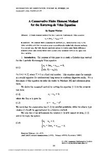
Figure 1: Configuration for smooth solution. Free flow regions left and right separated by a porous medium. Inflow and outflow boundary conditions left and right, slip at top and bottom.

level 2 3 4 5 6 7

uS error 1.3e-1 3.6e-2 1.0e-2 2.7e-3 7.1e-4 1.8e-4

rate — 1.83 1.81 1.90 1.94 1.96

uD error 3.4e-2 4.1e-3 9.9e-4 2.5e-4 6.4e-5 1.6e-5

rate — 3.02 2.07 1.98 1.97 1.98

pS error 1.4e-0 2.2e-1 5.2e-2 1.3e-2 3.4e-3 8.5e-4

rate — 2.74 2.04 1.98 1.98 1.98

pD error 5.1e-1 6.6e-2 1.6e-2 4.1e-3 1.1e-3 2.7e-4

∇·u rate — 2.94 2.03 1.97 1.98 1.98

2.4e-12 1.8e-12 7.0e-13 7.5e-13 1.5e-12 1.3e-12

Table 2: Intrinsic mean quadratic errors and convergence rates for the smooth problem solved with the RT1 /Q1 -element pair (ν = 1, K = 10−2 ).

First, we choose a problem with a smooth solution to show that the convergence rates are optimal with respect to mesh size. To this end, consider a geometry resembling flow through a porous filter as in Figure 1. We choose a quartic inflow and outflow profile on the left and right boundaries of the domain (noslip), such that ux and ∂y ux vanish at the upper and lower boundaries. Thus, we are consistent with the slip boundary condition on the top and bottom and the solution exhibits only mild singularities in the corners. Since all flow has to go through the filter in the center, the flow speed there is asymptotically independent of K as K tends to zero. Results for the pair RT1 /Q1 -element and permeability K = 10−2 are reported in Table 2. Since the exact solution is unknown, we present the L2 -norm of intrinsic errors obtained by taking the difference d` between numerical solutions on consecutive grid levels ` − 1 and `. The intrinsic convergence rates are obtained from these by the formula r` = log2 (d`−1 /d` ). Note that in case of geometric error reduction (constant convergence rates), the intrinsic error is equivalent to the standard error and only differs by a factor. The table shows, that in spite of the fact that the energy norm involves the derivatives of uS and the field uD itself, the mean quadratic errors of both converge with the optimal order 2. The same is true for the pressure in both subdomains. Thus, we conclude that the scheme is well balanced and convergence in the subdomains

10

paper.tex

1808

2009-08-17

15:42:44Z

kanschat

degree RT2

RT3

RT4

level 3 4 5 6 3 4 5 6 3 4

uS 1.61 2.82 2.97 3.00 3.73 3.80 3.85 3.88 4.05 4.03

uD 3.13 3.26 3.12 3.04 4.36 3.91 4.13 4.33 5.50 5.07

pS 1.92 2.29 2.38 2.42 3.60 3.24 3.10 3.04 3.03 3.00

pD 2.99 3.04 3.03 3.01 4.36 4.00 3.99 4.00 5.32 4.98

Table 3: Intrinsic convergence rates for higher order elements (ν = 1, K = 10−4 ).

Figure 2: Intrinsic velocity error distribution for RT4 /Q4 , exhibiting the weak corner singularities.

is not impeded by the coupling. The boundary conditions in this particular example were chosen such that the solutions for velocity and pressure are smooth. In Table 3, we show intrinsic convergence rates for higher order elements. The observed rates for the velocities are k + 1 as predicted; the reduced orders for uS with RT4 are due to lack of regularity of the solution (see Figure 2). The pressure pD exhibits order k + 1, as predicted by the theory for the Raviart-Thomas element for the mixed Laplacian. The convergence rate for the pressure pS confirms our analysis. We note that trivially the order of convergence of the global pressure corresponds to our error estimates. Next, we study the robustness of the errors with respect to the permeability K. Figure 3 clearly shows robustness of the relative error of the Stokes solution with respect to permeability. The relative error of the Darcy solution decays

11

paper.tex

1808

2009-08-17

15:42:44Z

kanschat

10-1

10-1

K=10-0 K=10-1 K=10-2 K=10-3 K=10-4 K=10-5

-2

10

10-3

10-2

10-4

10-3

10-5

10-4

10-6 10-7

K=10-0 K=10-1 K=10-2 K=10-3 K=10-4 K=10-5

3

4

5

6

7

10-5

8

3

4

5

6

7

8

Figure 3: Relative errors of uD (left) and uS (right) depending on refinement level for different permeabilities K.

Figure 4: Setup for flow in a river bed. The Stokes region is on top and the Darcy region on the bottom. Slip conditions left, right and bottom, noslip at the top.

linearly with permeability. This is caused by the fact that the norm of uD is nearly independent of K (all flow has to go through the filter), but the error scales with K −1 . In a second test, we consider an idealized flow in a river bed as depicted in Figure 4. This example differs from the previous in that the flow speed in the porous medium depends strongly on the permeability; for small permeabilities linearly. Since the flow is driven by the flow in the Stokes subdomain, where errors are expected to be independent of permeability, we expect the absolute errors of the Darcy velocity to reduce if K tends to zero. Nevertheless, since the solution there diminishes as well, this prediction might be wrong for the relative error. Indeed, in our experiment the absolute error on fine meshes behaves like K 1/2 , such that the relative error grows with K −1/2 . This is confirmed by Figure 5. Finally, we confirm that the method is strongly conservative. To this end, consider the configuration in Figure 6. The left half of the domain is the freeflow part with Stokes equations, a quadratic inflow profile and no-slip boundary conditions. The Darcy part on the right has slip conditions on the top and

12

paper.tex

1808

2009-08-17

15:42:44Z

kanschat

100

100

K=10-0 K=10-1 K=10-2 K=10-3 K=10-4 K=10-5 K=10-6

10-1 10-2

10-1 10-2

10-3 10-4

K=10-0 K=10-1 K=10-2 K=10-3 K=10-4 K=10-5 K=10-6

10-3

3

4

5

6

7

10-4

8

3

4

5

6

7

8

Figure 5: Relative errors of uD (left) and uS (right) in the river bed example depending on refinement level for different permeabilities K.

Figure 6: Configuration for mass conservation test. The thick boundary on the left half of the domain indicates no-slip, the dashed boundary on the right prescribed pressure p = 0.

bottom and pressure boundary condition p = 0 on the right. Accordingly, the normal flux u · n on the right boundary is a result of the computation. The velocity and pressure solution for this problem are shown in Figure 7. Since the strong normal boundary conditions on top and bottom assure that no mass is lost there, we use the difference of the integrals of the normal flux over the left and right boundaries, respectively, to demonstrate the conservation property of our method. With an incoming flux integral of 4/3, the results displayed in Table 4 show clearly that the mass flux error is close to the computational accuracy and thus confirms the strong conservation property of the method. 6. Conclusions We presented a uniform finite element method for the coupling of Stokes and Darcy flow. By the use of divergence-conforming elements, exact mass conservation is guaranteed. We presented an error norm estimate which is optimal with respect to the approximation spaces, but suggests an imbalance between 13

paper.tex

1808

2009-08-17

15:42:44Z

kanschat

Figure 7: Velocity field and pressure isolines for the mass conservation test with K = 10−4 .

level 2 3 4

K = 10−2 1.4e-08 2.5e-10 4.5e-10

K = 10−4 8.5e-10 2.7e-10 1.2e-09

K = 10−6 1.2e-09 5.1e-11 4.7e-09

Table 4: Mass flux difference between inflow and outflow side of the domain.

the subdomains. The results of the numerical experiments on the other hand indicate, that the the scheme is indeed well balanced and convergence orders in L2 are the same for the Stokes and the Darcy part. The proof of this convergence requires more involved analysis and will be postponed to a future article. Acknowledgments The numerical results in this article were produced using the deal.II finite element library [5]. References [1] Arbogast, T., Brunson, D., 2007. A computational method for approximating a Darcy-Stokes system governing a vuggy porous medium. Computational Geosciences 11, 207–218. [2] Arnold, D. N., 1982. An interior penalty finite element method with discontinuous elements. SIAM J. Numer. Anal. 19 (4), 742–760. [3] Arnold, D. N., Boffi, D., Falk, R. S., 2002. Approximation by quadrilateral finite elements. Math. Comput. 71, 909–922. [4] Arnold, D. N., Brezzi, F., Cockburn, B., Marini, D., 2001. Unified analysis of discontinuous Galerkin methods for elliptic problems. SIAM J. Numer. Anal. 39 (5), 1749–1779. 14

paper.tex

1808

2009-08-17

15:42:44Z

kanschat

[5] Bangerth, W., Hartmann, R., Kanschat, G., 2007. deal.II — a general purpose object oriented finite element library. ACM Trans. Math. Softw. 33 (4). [6] Beavers, G. S., Joseph, D. D., 1967. Boundary conditions at a naturally impermeable wall. J. Fluid. Mech 30, 197–207. [7] Brezzi, F., Douglas, J., j., Fortin, M., Marini, D., 1987. Efficient mixed finite element methods in two and three space variables. RAIRO Mod´el. Math. Anal.Num´er. 21, 581–604. [8] Brezzi, F., Douglas, J., j., Marini, D., 1985. Two families of mixed finite elements for second order elliptic problems. Numer. Math. 47, 217–235. [9] Brezzi, F., Fortin, M., 1991. Mixed and Hybrid Finite Element Methods. Springer. [10] Burman, E., Hansbo, P., 2005. Stabilized Crouzeix-Raviart elements for the Darcy-Stokes problem. Numerical Methods for Partial Differential Equations 21, 986–997. [11] Burman, E., Hansbo, P., 2007. A unified stabilized method for Stokes and Darcy’s equations. J. Computational and Applied Mathematics 198 (1), 35–51. [12] Cockburn, B., Kanschat, G., Sch¨otzau, D., 2005. A locally conservative LDG method for the incompressible Navier-Stokes equations. Math. Comput. 74, 1067–1095. [13] Cockburn, B., Kanschat, G., Sch¨otzau, D., 2007. A note on discontinuous Galerkin divergence-free solutions of the Navier-Stokes equations. J. Sci. Comput. 31 (1–2), 61–73. [14] Discacciati, M., Miglio, E., Quarteroni, A., 2002. Mathematical and numerical models for coupling surface and groundwater flows. Appl. Numer. Math. 43 (1-2), 57–74, 19th Dundee Biennial Conference on Numerical Analysis (2001). [15] Gatica, G., Meddahi, S., Oyarzua, R., 2009. A conforming mixed finiteelement method for the coupling of fluid flow with porous media flow. IMA Journal of Numerical Analysis 29, 86–108. [16] Girault, V., Raviart, P.-A., 1986. Finite element approximations of the Navier-Stokes equations. Springer. [17] Girault, V., Rivi`ere, B., 2007. DG approximation of coupled Navier-Stokes and Darcy equations by Beaver-Joseph-Saffman interface condition. SIAM J. Numer. Anal.

15

paper.tex

1808

2009-08-17

15:42:44Z

kanschat

[18] Hansbo, P., Larson, M. G., 2002. Discontinuous Galerkin methods for incompressible and nearly incompressible elasticity by Nitsche’s method. Comput. Methods Appl. Mech. Engrg. 191, 1895–1908. [19] Hanspal, N., Waghode, A., Nassehi, V., Wakeman, R., 2006. Numerical analysis of coupled Stokes/Darcy flows in industrial filtrations. Transport in Porous Media 64 (1), 1573–1634. [20] J¨ ager, W., Mikeli´c, A., 2000. On the interface boundary condition of Beavers, Joseph, and Saffman. SIAM J. Appl. Math. 60 (4), 1111–1127 (electronic). [21] Kanschat, G., 2007. Discontinuous Galerkin Methods for Viscous Flow. Deutscher Universit¨ atsverlag, Wiesbaden. [22] Layton, W. J., Schieweck, F., Yotov, I., 2003. Coupling fluid flow with porous media flow. SIAM J. Numer. Anal. 40 (6), 2195–2218. [23] Nassehi, V., 1998. Modelling of combined Navier-Stokes and Darcy flows in crossflow membrane filtration. Chemical Engineering Science 53 (6), 1253– 1265. [24] Raviart, P.-A., Thomas, J. M., 1977. A mixed method for second order elliptic problems. In: Galligani, I., Magenes, E. (Eds.), Mathematical Aspects of the Finite Element Method. Springer, New York, pp. 292–315. [25] Rivi`ere, B., 2005. Analysis of a discontinuous finite element method for the coupled Stokes and Darcy problems. Journal of Scientific Computing 22, 479–500. [26] Rivi`ere, B., Wheeler, M. F., Girault, V., 2001. A priori error estimates for finite element methods based on discontinuous approximation spaces for elliptic problems. SIAM J. Numer. Anal. 39 (3), 902–931. [27] Rivi`ere, B., Yotov, I., 2005. Locally conservative coupling of Stokes and Darcy flow. SIAM J. Numer. Anal. 42, 1959–1977. [28] Saffman, P., 1971. On the boundary condition at the surface of a porous media. Stud. Appl. Math. 50, 292–315.

16

paper.tex

1808

2009-08-17

15:42:44Z

kanschat