European Congress on Computational Methods in Applied Sciences and Engineering ECCOMAS 2004 P. Neittaanmäki, T. Rossi, K. Majava, and O. Pironneau (eds.) W. Rodi and P. Le Quéré (assoc. eds.) Jyväskylä, 24—28 July 2004
A BOUNDED CONTROL VOLUME HYBRID FINITE ELEMENT METHOD FOR SUBSURFACE MULTIPHASE FLOW SIMULATIONS
Andrey A. Mezentsev*, Stephan K. Matthai*, Christopher C. Pain* and Matthew D. Eaton* *
Department of Earth Sciences and Engineering Imperial College London, Exhibition Road, London SW7 2AZ, U.K. e-mail:
[email protected], web page: http://www.ese.ic.ac.uk
Key words: Control Volume Finite Element method, Hyperbolic Diffusion-advection equation, Free Form Geometry, Hybrid Mesh Abstract. This paper develops hybrid mesh generalisation of a new implicit high order in space and time 3D Control Volume – Finite Element transport method applicable for single and multiphase flow simulations on complex geometry. It utilises unstructured spatial hybrid finite element meshes to capture free form geometry of geological objects with multiple material interfaces. Precise geometry definition is achieved with the novel in subsurface simulation 3D free-form Non-Uniform Rational B-spline models in CAD Boundary Representation with full model topology. The finite element framework is used as the basis for the node centred control volume discretisation. The finite elements are subdivided into control volume sectors, using systematic tessellation in the iso-parametric space of each type of element, found in the mesh. A generic iso-parametric formulation for the control volume surface and volume numeric integration is presented. Advantages of the new transport are demonstrated on a number of single and multiphase transport simulations for very complex fractured reservoir geometry.
1
Andrey A. Mezentsev, Stephan K. Matthai, Christopher C. Pain and Matthew D. Eaton.
1
INTRODUCTION
Computer simulation of multiphase flow on discrete realistic geometry in subsurface is a challenging problem. Mathematically it is governed by a set of non-linear convection– diffusion type equations [1-4] of and takes place in extremely complex geometrical domains [5-8]. Geological structures, such as faults and fractures influence greatly the pattern of flow in subsurface with major implications for flow pattern in fractured petroleum reservoirs [5-8], commonly simulated with a continuum, dual-porosity or dual-permeability approach. This technique is widely applied, but it is now recognized that it is not possible to capture flow behaviour accurately through these method [5-8]. Numerical techniques such as the Finite Element (FE) and/or the Control Volume (CV) methods are used for accurate discretisation of the transport equations on realistic geological geometry [4-9]. But complexity of geometry with numerous material interfaces requires unstructured FE or CV mesh in 3D [1-4]. Volumetric discretisation of fractures is novel for the subsurface flow simulation (e.g. [6-9]). In this work we develop a framework for a generic 3D Control Volume – hybrid (in the mesh generation community known as mixed element type) Finite Element Method (CVHFEM) for the simulation of transport phenomena in fractured rocks. The key points of new method are realistic definition of the geometry as fully volumetric entities and application of the Control Volume Hybrid Finite Element method on unstructured meshes. Volumetric entities of the geometry - the solids - are defined in Computer Aided Design (CAD) spline Boundary Representation form [9] dividing space into watertight geometric sub-regions. Fractures and other material interfaces are considered as solids as well. Many complex fluid flow problems for free form geometries have been solved with the unstructured FEM and the CVM [1-4]. The CVM is particularly popular because it leads to an exact satisfaction of the conservation laws [2,3]. The FEM and CVM have much in common: both are integral formulations and use shape functions for mesh discretisation and interpolation [1-4]. The Control Volume Finite Element node centered method (CVFEM) (Baliga and Pantakar [10,11], Durlofsky [14], Pain et al. [12,13], Mezentsev et al. [19]) combines geometry conforming capabilities and high order accuracy of the FEM and conservative formulation of the CVM, which makes it very attractive for efficient hyperbolic transport simulations in geometrically complex fractured petroleum reservoirs. Baliga and Pantakar [10,11] introduced the method for linear triangle FEs. Subsequently, the method was extended to other elements types in single element type formulations. Two extremely difficult problems need to be addressed during development of the discrete fractured reservoir models: the problem of complex meshing geometry [10,17,18] and complex physics of the flow [4,5]. Complexities of spatial discretisation (meshing) inside volumetric fractures have prompted researchers [5-8] to use simplified lower spatial dimension representation of fractures as surfaces and lines. Dimensionality of the problem is significantly reduced, but it is not possible to represent certain flow effects without internal degrees of freedom inside the spatial discontinuities. Though the complexity of geological geometry and topology of the fractures are fully acknowledged in [5-8], the full problem of the adequate 3D geological geometry description for further meshing is still underestimated.
2
Andrey A. Mezentsev, Stephan K. Matthai, Christopher C. Pain and Matthew D. Eaton.
On the other hand, the complexity of the physics in discrete multiphase flow simulation is understood well and the main problem here is to address correctly the aspects of numerical solution [4]. In this paper a new bounded implicit high order in space and time numerical method for the CVHFEM transport simulation on free form spline models of geological objects is developed. First we describe challenges of spatial discretisation of fractured geometry by 3D hybrid FE meshes. Second, we give a brief description of the governing equations and their discretisation by the CVHFEM. Third, we develop a generic method of the volume and surface numeric integration for unified iso-parametric formulation. Fourth, we demonstrate results of the method application to the simple and realistic transport models. 2
SPATIAL DISCRETISATION
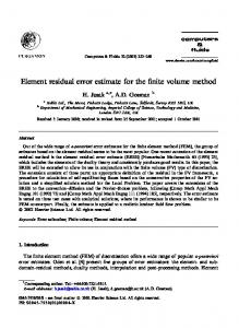
2.1 Meshes for realistic complex geological objects The mesh needs to capture complex geometric features of the typical geological geometry. For the fractures shown in Figure 1, the ratio of the length to average aperture is around 103 107. All fractures have variable aperture and are free form 3D volumetric objects embedded in a rock matrix. Fractures intersect at small angles and in size can vary of many orders of magnitude. Geometric models for mesh generation should represent volumetric entities with high aspect ratio and provide the possibility to capture small-angle intersections. They must also be capable of handling of thousands of volumetric objects at a time. In this situation simplified poly-line geometric models used in [5,6,7] cannot represent desired features. It is important, that Bogdanov et al. [7] pointed on a negative role of the geometric round-off errors in the intersection regions of multiple fractures, represented by surfaces, but did not propose a solution. In our opinion, this problem appears due to the absence of the relevant topology information in the geometric model and accumulation of the geometric approximation errors. The 3D meshing requires consistency of the internal sub-volumes in the model, excluding gaps and overlaps [9,20]. We use for description of geological geometry the Computer Aided Design (CAD) free form Non-Uniform Rational B-spline (NURBS) models with Boundary Representation of the topology [9]. Application of the chosen CAD format permits to capture free-form geometry with high relative accuracy (up to 1E-9). Standard CAD tools can be used for geometry editing, and the FE mesh can be generated directly using the CAD model. Our model contains comprehensive hierarchy of geometric entities and their relation to each other, forming the topological tree from vertex to the whole model. That is very important, as many errors in 3D mesh generation are attributed to absence of topological information during CAD import into the mesh generator [20]. Simulation of multiphase flow inside volumetric fractures (Figure 2) requires a refined 3D mesh and meshing is a significant problem [10,17,18]. Theoretically it is possible to discretise space inside fractures with tetrahedral elements similar to the method used by Bogdanov et al. [7] for subsurface flow simulations, but the requirement of internal degrees of freedom necessitates a small size of the elements and brings their overall number to extremely large numbers. High aspect ratio elements are likely in our applications, and we are interested in
3
Andrey A. Mezentsev, Stephan K. Matthai, Christopher C. Pain and Matthew D. Eaton.
interpolation properties of high aspect ratio elements. In general, trilinear hexahedral meshes provide a better approximation than corresponding tetrahedral meshes with the same number of degrees of freedom due to better interpolation properties of the hexahedral element [21]. So the all-hexahedral mesh inside the fractures could solve the meshing problem. However, automatic all-hexahedral meshing for free form geometry is extremely difficult [1,9] and therefore the multi-block structured method is mostly used (Jenny et al. [8]) in geological applications. For the complex geometry, depicted at Figure 2 multi-block meshing requires a lot of human intervention and can be hardly automated [17].
Figure 1. Typical Fractured Rocks Pattern (Kilve, Somerset, United Kingdom).
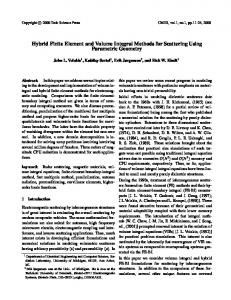
Figure 2. Free form NURBS CAD model of the rocks above. Typical fracture length is 15 m and the aperture is around 0.01 m, numerous intersection curves and sharp intersection angles between the fractures are shown. Geometry is mapped and drafted by Dr. M. Belayneh, Imperial College.
Hex-dominant meshes can be automatically generated using initial all-tetrahedral mesh, and this approach is called indirect [9,18]. The simple idea of the decomposition of tetrahedron to four hexahedrons proved to be unusable due to bad quality of the mesh and increased number of the mesh nodes. The other indirect method uses unification of 12 tetrahedral elements to one hexahedron following certain quality criterion for the conversion, aspect ratio of the element, for example [9]. Near the geometrical constraints of the model tetrahedrons cannot be converted at prescribed quality and are kept without changes. Prism and pyramid elements are used to interface tetrahedrons to hexahedrons. (See Table 2). To use hybrid mesh for the node-
4
Andrey A. Mezentsev, Stephan K. Matthai, Christopher C. Pain and Matthew D. Eaton.
centered CVPEM we require a generic methodology for discretisation by virtual CV cells for hybrid unstructured meshes. This paper develops such a methodology. 3
METHODS
This section presents the governing equations and their discretisation in space and time. This includes the presentation of our new conservative transport scheme, and a brief discussion of the new iso-parametric numeric integration method for the CVHFEM transport scheme. 3.1 Governing equations Like Durlowsky [14] or Huber and Helmig [4] we compute transient fluid pressure diffusion and immiscible displacement of slightly compressible phases in a sequential manner: First, an elliptic-parabolic pressure equation is solved to obtain the flow velocity, vt, from the gradient in fluid pressure, p, and the total fluid mobility, λt, via Darcy's law, taking into account buoyancy contributions due to fluid density, ρ: v t = − λ t [∇ p + g ρ ] = − λ t ∇ p r (1) In this expression, the vector g is the acceleration due to gravity. The gradient of pr is derived from experimentally determined pr - saturation relationships varying among rock types. Conservation of total fluid volume in slightly compressible flow requires that the divergence of the total flow field is zero except for where local fluid sources or sinks, q&exist (for instance wells), note that q is a proportional volume per volume and hence dimensionless term, q&= ∂q / ∂t : ∇vt − q&= 0 (2) By substituting Darcy's law for vt we obtain: − ∇ ⋅ λ t ∇ p − q&= 0 (3) The total mobility, λt, requires a knowledge of the permeability tensor K, relative permeability multipliers for each phase, k ri , and their viscosities µ i (where i = n,w) for wetting and non-wetting phases:
k k λ t = K rn + rw µw µn
(4)
The calculation of k ri multipliers relies on experimentally parameterized models like those of Brooks and Corey, van Genuchten and Sorey and Grant (1980), [4]. For transient pressure diffusion equation (3) becomes:
ct
∂pr = ∇ ⋅ λ t ∇ p r + q& ∂t
(5)
where the left-hand multiplier, ct, is the total system compressibility above the bubble point c t = φ (ψ w β w + (1 − ψ w )β n ) + (1 − φ )β s (6)
5
Andrey A. Mezentsev, Stephan K. Matthai, Christopher C. Pain and Matthew D. Eaton.
ct is a function of the individual compressibilities of the wetting, non-wetting and solid phases, β w , β n , β s , their saturations ψ i , and the porosity, φ i . ct determines the hydraulic diffusivity of the system, k p = λt / ct . The subscripts r in the pressure equation (5), denote the reduced fluid pressure (driving head pr) and average fluid density ρ r normalized by a reference density, ρ o ,
ρ r = ρ o − (ψ n ρ n + (1 − ψ
)ρ w )
(7) Thus, the actual fluid pressure, p, as required for the computation of equation of state properties like ρ or µ , is obtained from n
p = pr + ρo g
(8) Once the velocity distribution in the flow domain has been established we can calculate the immiscible displacement of the phases by solving a transport equation that must be formulated in terms of specific phase saturation. Only the transport of one phase need be computed because the sum of the transported phases is always equivalent to one. Buckley and Leverett (1942) [22] showed that, for piston-type displacement, the position of the saturation front can be calculated as a product of vt and the fractional flow, fi, of the phase i of interest: λi fi = (9) λn + λv This permits us to write the transport equation. ∂ψ i φ + ∇ ⋅ [ f i vt ] + ∇ ⋅ [λi f i∇pc ] + q& (10) i = 0 ∂t Unfortunately, equation (10) can be strongly hyperbolic. To moderate this, we can rearrange and expand it into a form that captures the capillary spreading of the saturation field by a diffusion term. ∂ψ i df dp φ = −vt ⋅ i ∇ψ i − f i∇ ⋅ vt − ∇ ⋅ λi f i c ∇ψ i + q& (11) iψ i = 0 ∂t dψ i dψ i In this approach, the divergence in the flow field of the phase i is accounted for by the
source or sink term f i ∇ ⋅ v t ⋅
df i and capillary spreading is treated as non-linear d ψ i
diffusion. Alternatively, we can directly compute capillary pressure gradients for phase i dp 2 Kλi ∇ p c = c K [λi ∇ψ i ] dψ i
(12)
and resulting phase velocity vi = f i Kλi +1∇p c . It can be added to the convective vt fi product, but needs to be accounted for in the divergence term. Like Durlowsky [14], or Hubert and Helmig [4] we employ linear FEs to discretise the pressure equation (3), using a complementary CV tessellation to achieve flux continuity and conservation of fluid volume (Figure 3).
6
Andrey A. Mezentsev, Stephan K. Matthai, Christopher C. Pain and Matthew D. Eaton.
Exact Solution Linear FEM Solution
f(x)
Element 1
Element 2
Element 3
Finite Volume
Node 1
Node 2
X
Derivative of Linear FEM Solution, e.g., pf gradient
Figure 3. 1D dual mesh CV finite element discretisation of a Darcian fluid flow. Fluid pressure is discretised using the piecewise linear FE basis functions with piecewise constant pressure derivative that is discontinuous across element boundaries, but exact at element centers, where it is used to compute the surface normal fluxes in and out of CV cells. CV discretisation achieves flux continuity for 1st order FE discretisation.
In the CVFEM approach FEs and CVs assume a complementary pressure derivative. For two steadily differentiable functions, f and g, that define a two-dimensional velocity field, F, ( ∇ ⋅ F = ∆ g − g ∆ f ), Gauss' integration theorem states the equivalence between a volume and a surface integral over a real domain of interest, A, of the actual functions versus their derivatives normal to the domain boundary:
∫ (∆g − g∆f )dV = ∫
∂A
A
( fn ⋅ ∇g − gn ⋅ ∇f )dS
(13)
Therefore, a CV discretisation that places cell boundary segments (hereafter called facets) into the FEs, where the FE interpolation functions are continuous, is all that is needed to correctly integrate the discontinuous velocity field that arises from the differentiation of the piecewise linear element interpolation functions. With these node-centered CVs we can directly solve the conservation law. ∇⋅F = 0 (14) A subdivision of the all types of element in the hybrid mesh into CV sectors, as first proposed by Baliga and Patankar [10]. Similar to Durlowsky [14] we do not actually store the CV mesh, but accumulate corresponding CV stencils directly in a solution matrix. The main difference to earlier twodimensional approaches restricted to triangles (Baliga and Patankar for example [10,11]), is the complete generality of our new CV discretisation. It applies to models where CVs are composed of arbitrary combinations of 3D FEs in as much as this is required to capture complex geometry. Furthermore, since our new scheme is based on iso-parametric FEs, progressive deformation of the mesh in coupled models does not compromise the accuracy of CV integration. Table 2 shows an example of such a hybrid FE mesh in which fractures are represented by large aspect-ratio hexahedral and prism elements, mesh-size gradients are accomplished using tetrahedral and triangular elements, and uniform volumes are represented by hexahedra. This memory efficient representation leads to relatively regular distribution of nodes in space.
7
Andrey A. Mezentsev, Stephan K. Matthai, Christopher C. Pain and Matthew D. Eaton.
An important observation that has been ignored by earlier works on the FEM-CV approach is, that the overall domain integral over a primary distributed point variable (for instance saturation) discretised with point-centered piecewise constant CVs is not exactly the same as for piecewise linear FEs whose nodes coincide with the points. Therefore, a transformation is required to map CV-discretised variables to FEM nodes in order to interface FE with CV computations in a consistent manner.
∫
FV
[Ψˆ (x , y , z , t ) − Ψ (x , y , z , t )]_ dV N
Ψˆ ( x , y , z , t ) =
∑
Ψ (x , y , z , t ) =
N
FE
N
i =1
∑
i
FV
M
i =1
i
= 0 ∀ i ∈ [1 ... n ]
(15)
(x , y , z )ψˆ ( t )
(16)
( x , y , z )ψ
(17)
(t )
The equivalence of variable Ψ in the CV and the FE discretisation can be imposed by solving the global matrix equation: (18) ψˆ = B −1 P Ψ (t ) where (19) B = ∫ N i N j dV V
P
=
∫
V
(20)
N i M j dV
This achieves the transformation of ψ back into the FE reference frame once a transport step has been carried out. For further details we refer the reader to [12,19]. 3.3 spatio- temporal integration: solution procedure
The pressure equation (5) is solved using a standard Bubnov-Galerkin FE method. Trilinear element interpolation functions Ni are used to integrate fluid pressure in space and are equivalent to the nodal weights Wi. The fluid pressure is evolved using an implicit backward-Euler integration of time.
[∫ N ∫
N
T
T
c t NdV c t NdV
+ ∆ t ∫ DN
(p t )+
T
λ t DNdV
( ∫N
∆t −
T
]( p
t+∆t
)=
λ t g ρ r N z dV + q
)
(21)
Here N T and DN T represent the interpolation function vector and matrix of their spatial derivatives. The mass matrices are lumped. Square and rounded brackets have been introduced into equation (21) to discern terms accumulated into the global solution matrix versus the right hand vector, respectively. To find a unique solution to (21), Dirichlet boundary conditions must be specified somewhere in the computational domain. Capillary pressure gradients for phase i can be computed directly using the approach described above: dpc T T (22) ∫ DN Kλi DNdV = dψ i ∫ DN DNNψ i dV
8
Andrey A. Mezentsev, Stephan K. Matthai, Christopher C. Pain and Matthew D. Eaton.
The CV discretisation of the transport equation (11) yields a series of volume and surface integrals over the boundaries of each CV as well as volume integrals for distributed sources and sinks and the bijective mapping. CV integrals are expressed in terms of the piecewise constant CV interpolation functions Mi as was discussed above. For each FE, there are as many internal surfaces and integral contributions to finite volumes as there are connections between nodes. This set constitutes the characteristic CV stencil associated with the element, which is accumulated into a global solution matrix A and right hand vector b. The CV integrals for a first-order accurate upwind scheme are ∂ψ i dV + ∫ n ⋅ vtψ c dS + ∫ n ⋅ vtψ u dS − ∫ M i qdV = 0 φ∫ Mi (23) FV FVout FVint FV ∂t Here in an out denote the ingoing and outward fluxes with regard to the CV cell, i, respectively. The subscripts, u, c, d refer to the far-field upstream, current, and downstream finite volumes. For the flux-limited higher-order CV discretisation of the transport equation we use the following integral form: ∂ψ i φ∫ Mi dV + ∫ n ⋅ v tψ~ k dS − ∫ M i qdV = 0 (24) FV FVt FV ∂t where the flux-limited higher-order finite-element approximation ψ~k , replaces the upwind approximation ψ u (equation 23) and the source q also includes flow-field related divergence terms. Due to the flux limiting, equation (24) is now non-linear, and needs to transformed into a linear system of equations before it can be solved. We achieve this by means of a Picard iteration in which the first-order upwind solution serves as a guess of ψ t + ∆t at iteration level, p+1. The solution is iteratively improved until changes between iteration levels diminish below a specified tolerance. We would like to emphasis the following observation. As it was pointed out by Leveque [3], full potential of the high order spatial discretisation can only be exploited up to the stability limits only in conjunction with the high order temporal discretisation, and therefore we developed the Θ− limited second order time stepping for our method. For further details of our high order spatial and temporal discretisation we refer the reader to [12] and [19]. The researchers largely ignore the other observation, ensuring the efficiency of the method, the generality of the methodology of the numeric integration procedures for a hybrid mesh in (23) and (24), which we will discuss here in detail. 3.4 Volume and surface integration for the CVHFEM
(
)
We use the definition of the FE [1]. It is a triple K ,P, ∑ of a closed connected set
K ∈ ℜ with non-empty interior and Lipschitz - continuous boundary, a finite-dimensional space P of real-valued functions, and a set of linear forms Σ, the degrees of freedom. We introduce a fictious parametric space for each type of element in the mesh and reference element (K ′, P ′, ∑ ′) in it. In case of linear FE, a trilinear invertible bijective mapping M k : K ′ → ℜ n relates physical (x, y, z) to the parametric (r, s, t) coordinates. Invertibility of n
9
Andrey A. Mezentsev, Stephan K. Matthai, Christopher C. Pain and Matthew D. Eaton.
the mapping implies usage of the incomplete polynomial space of a Lagrangian formulation. In case of the complete polynomial space it is not possible to use mappings for a pyramid element, which has non-invertible mapping M k [23]. So our formulation differs from that in the complete polynomial space interpolation and we need to establish the mappings between the CV sector in physical space and its parametric representation. This permits to simplify the calculation of the basic CV and FE integrals and enables application of high order curvedsided FEs. For this purpose, each CV sector is treated as a topological hexahedron for volume elements and as quadrilateral for surface elements. The FEs are subdivided by facets to the CV sectors (see Table 1 and Figure 2 for nomenclature). Sectors constitute the virtual CV around each node and are delimited by facets spanning between the following characteristic points inside the FE: the FE node, midpoints of the element’s edges containing the node, barycentre of the element and centres of the element’s faces the node belongs to (Figure 4). The consistency of the volume subdivision is maintained, as we ensure topologically quadrilateral/hexahedral division pattern for the elements both with triangular and quadrilateral faces. The composite mapping (Μ ΜS) between the parametric and physical space of the CV sector consists of two consecutive trilinear mappings (Μ Μ1 and Μ2) and is performed for all types of elements in the hybrid mesh (Figure 5). 1. The hexahedral CV sector in physical space (x,y,z) is mapped to the hexahedral sector in local coordinates of the FE (r,s,t), constituting a trilinear mapping Μ1 with the following Jacobian J1 : ∂r ∂s ∂t ∂x ∂x ∂x ∂r ∂s ∂t J1 = (24) ∂y ∂y ∂y ∂r ∂s ∂t ∂z ∂z ∂z 2. The hexahedral sector in local coordinates (r,s,t) is mapped to the unit parametric cube with local coordinates (r’,s’,t’) . This constitutes trilinear mapping Μ2. with the corresponding Jacobian J2 : ∂r ' ∂s ' ∂t ' ∂r ∂r ∂r ∂r ' ∂s ' ∂t ' J2 = (25) ∂s ∂s ∂s ∂r ' ∂s ' ∂t ' ∂t ∂t ∂t
10
Andrey A. Mezentsev, Stephan K. Matthai, Christopher C. Pain and Matthew D. Eaton.
Element
Number of nodes
Number of facet walls
Tetrahedral
4
6
Pyramid
5
8
Prism
6
9
Hexahedral
8
12
Figure
Table 1. Hybrid Finite Elements decomposition into Finite Volume sectors.
11
Andrey A. Mezentsev, Stephan K. Matthai, Christopher C. Pain and Matthew D. Eaton.
Figure 4. Nomenclature of tetrahedral FE subdivision to CV sectors.
Figure 5. Composite mapping for the Control Volume sector.
12
Andrey A. Mezentsev, Stephan K. Matthai, Christopher C. Pain and Matthew D. Eaton.
The position of the Gaussian volume and surface integration points are given in local coordinates of the (r’,s’,t’) parametric space and mapped to (r,s,t) using Μ2. The overall mapping between a reference unit cube in (r’,s’,t’) and the CV hexahedral sector in physical space (x,y,z): ΜS = Μ1 Μ2 (26) is needed to obtain the weights for surface integration over the facet and volume integrations over the sector. This numerical integration can be carried out in parametric space (r’,s’,t’) using the standard 3D Gauss product rules [1]: 1 1
∫∫
−1 −1
1
∫ F ( r , s , t )drdsdt =
−1
1
1
1
∫ ds ∫ dr ∫ F ( r , s , t ) dt ≈
−1
1 i
−1
1 j
−1
p1
p2
p3
∑∑∑w
1 i
w 1j w 1k F ( ri , s j , t k ) (27)
i =1 j =1 k =1
1 k
The Gauss integration weights w w w are determined in a two-step procedure and are defined as follows (Figure 5): wi1 = wi2 det J 2 w1j = w 2j det J 2 w1k = wk2 det J 2 (28) where det J 2 is the determinant of the Jacobian matrix of the mapping Μ2. Using the once calculated weights in formula (27) we can perform any numeric integration for volumetric elements and surface facets. For quadrilateral facets in physical space (x,y,z) we establish mapped quadrilateral facets first in the parametric space (r,s,t) of the FE, and then for a unit iso-parametric quadrilateral in (r’,s’,t’). The volume numeric integration algorithm will be as follows: For all integration points: Interpolate transport variable to the tabulated Gaussian integration points p1, p2, p3 of the given CV facet or sector in the parametric space (r,s,t) of the FE, using the FE interpolation functions(8); For the tabulated Gaussian integration points p1, p2, p3 calculate the determinant J1 of the Jacobian transformation matrix between physical and parametric space (24); Multiply the interpolated variable (step 1) with the determinant of the Jacobian J1 (step 2) and weights wi1 w1j w1k at the tabulated Gaussian integration points in space (r,s,t) to obtain the contribution of the given integration point; Sum the contribution from integration points. End Loop Integral = Sum An interesting implication of the topological complexity of the pyramid element decomposition to hexahedrons [18] is that the CV sector at the apex of the pyramid is an octahedron. We decompose this into two hexahedrons (Table 1, pyramid element) and combine their contributions to that sector. To identify tabulated positions of the surface and volume integration points in parametric spaces (r,s,t) of different FE types and their composite weights, for each local node of all FE
13
Andrey A. Mezentsev, Stephan K. Matthai, Christopher C. Pain and Matthew D. Eaton.
types the following steps were taken: • Tabulation of the positions of corner points of the hexahedral sector in the parametric space (r,s,t) of each FE. This sector is represented by the unit parametric cube in space (r’,s’,t’) (Figure 5); • Definition of the hexahedral shape functions for iso-parametric representation of the sector; • Definition of the integration point positions using known parametric coordinates in space (r’,s’,t’); • Definition of the shape functions derivatives, Jacobian J 2 and it’s determinant for mapping Μ2 ; • Calculation of the Gauss integration weights wi1 w1j w1k using (28); These steps were carried out only once and later tabulated integration points positions and composite integration weights are used in the procedures for numeric volume and surface integration. 4
RESULTS
We have applied the developed CVHFEM method to simulations of the single and multiphase flow on extremely complex free-form geological geometries, automatically discretised with hybrid unstructured meshes. The method is used in the generic objectoriented FE code CSP4.0, developed by S.Matthai et al. [16] Table 2 gives an outline of the complexity of our meshes, generated by the ICEM CFD (Ansys Inc.) and Mezegen (A. Mezentsev) [24] automatic hybrid mesh generation codes. ICEM CFD uses octree method for generation of the all-tetrahedral meshes, Mezgen uses constrained Delaunay method with efficient boundary recovery, proposed by Hassan and Weatherill (1997). Both meshers later convert all-tetrahedral mesh to hybrid, unifying 12 tetrahedrons to one hexahedron in geometrically unconstrained regions of the model. As per Table 2, hybrid meshes permit to significantly reduce memory requirements for the FE mesh and variables storage, giving the possibility to perform large CFHFEM simulations on the 32bit computers with the addresseble memory limitation of around 2 Mb. Note, that in Table 2, the mesh is presented by a thin cut through domain, exposing 3 layers of elements. The ratio parameter gives the ratio of number of elements to the number of nodes in the model. Model
Image
Tetrahedral
Hybrid
Cube in cube
Nodes: 257734
Nodes: 132655
(ICEM CFD)
Elements: 1532024
Elements: 141134
Ratio: 5.94
Ratio: 1.06
Memory: 539 Mb
Memory: 67 Mb
14
Andrey A. Mezentsev, Stephan K. Matthai, Christopher C. Pain and Matthew D. Eaton.
Irregular disk (Mezgen)
Fractured Reservoir (ICEM CFD)
Nodes: 8786
Nodes: 7039
Elements: 55301
Elements: 33132
Ratio: 6.29
Ratio: 4.71
Memory: 18.5 Mb
Memory: 11.5 Mb
Nodes: 169731
Nodes: 147167
Elements: 1106213
Elements: 703072
Ratio: 6.52
Ratio: 4.78
Memory: 370 Mb
Memory: 240 Mb
Table 2. Comparison of the mesh complexity for the same geometry.
a)
b)
c) d) Figure 6. Test of the step function advection on the hybrid mesh: a) 3D hybrid mesh of box geometry, Mezgen mesh generator, indirect method; b) First order CVHFE solution. Contours of concentration of step function are shown; c) High order in space/time CVHFE solution, time step 1.0*Courant number of the mesh; d) High order in space/time CVHFE solution, time step 10.0*Courant number of the mesh.
15
Andrey A. Mezentsev, Stephan K. Matthai, Christopher C. Pain and Matthew D. Eaton.
Figure 6 b) shows that the first-order accurate fully implicit and therefore very robust upwind scheme generally captures the advected step function profile, but it is highly diffusive and therefore unsuitable for the accurate advection of a passive tracer. On the other hand, Figure 6 c) shows that the high-order accurate fully implicit scheme with Θ-limiting captures the advected profile much more accurately, moreover, the application of the new time stepping permits to maintain high accuracy and physical realism even for large time steps as well (Figure 6 d)). This analysis indicates, that close to optimal results at CFL around 3.0. At such small CFL numbers, the bijective mapping is optimal even for highly irregular grids, the Picard iteration scheme converges in a few cycles, the slope limiter is phased in only weakly, and the Θ-limiting achieves higher-order accuracy in time in most of the model domain. For strongly increased CFL values (up to CFL 1,000) we have observed, that second-order accuracy reduces to first order in much of the simulation domain, the front begins to lag by one half of a CFL step (this is hard to verify since the front already is fairly diffuse), and, depending on the set tolerance, the Picard iteration may take more than 100 cycles to converge. If convergence is not monitored, an early termination of the iteration loop may lead to mild negative or positive oscillations ahead or behind the front, respectively. For the multiphase flow, the advantageous behavior of the developed scheme is due to the functional form of the fractional flow derivative, which implies that the front is selfsharpening and downstream flow beyond the shock front is suppressed. If the actual fractional flow is replaced by the characteristic shock speed, the first-order scheme is highly diffusive and therefore overshoots the proper location of the shock. For this reason it is better to apply the higher-order method to the saturation forecasting for time-increment - velocity products that exceed the grid Courant number (c.f., Figure 7).
a) b) Figure 7. Multiphase flow simulation (Brooks-Corey relative permeability model) in the three layer reservoir. Upper/lower layer – homogeneous with permeability 1e-12, porocity 0.2, middle layer free form fractured with matrix permeability 1e-14 and porocity 0.2, fracture permeability 1e-10. Oil/water viscosity ratio 1.0. Water injection at upper corner (a) or right corner of the model (b), initial oil saturation 0.95, model: 30x30x15 meters. a) Oil saturation profiles in fractured layer after 3.75 days of water injection, time step 3.0*Courant number. b) Characteristic Buckley-Leverett profile after 1.3 of water injection from the right.
16
Andrey A. Mezentsev, Stephan K. Matthai, Christopher C. Pain and Matthew D. Eaton.
While the simulations at large CFL numbers reveal a behavior of the higher-order accurate transport scheme that is far from ideal, the method still remains conservative, and retains at least first-order accuracy. Thus, when applied to strongly heterogeneous and adaptively refined discrete fracture model (Figure 7) with very tight global CFL constraints, the new scheme reveals its genuine superiority relative to Implicit for Pressure Explicit for Saturation (IMPES) methods. Figure 7 shows a solution for a contrived fracture model that includes geometrically challenging features like small-angle fracture intersections, cusps, and constrictions. Although the solution was computed for a global CFL value of 10, it is close to optimal over much of the fracture surface area. The more diffusive behavior at large CFL in the fast-flowing sub-regions of the model is offset by the increased refinement in these geometrically complex parts. The discrete fracture models are all characterised by a strong feedback between saturation and total mobility. This coupling is most pronounced when fracture permeability exceeds matrix permeability. In this case, at oil-water viscosity ratio near 1.0, water injection fronts tend to stabilize, because total mobility is reduced by up to an order of magnitude where fractures have a saturation around 0.5 near the front and the matrix is still oil saturated (e.g., Figure 7). At oil-water viscosity ratio of greater than 2, fronts in the same fractured media are characteristically unstable and finger widely in the flow direction. DISCUSSION
Preliminary testing of our new transport scheme to the general hyperbolic and specifically Buckley-Leverett equation [22] and fractured reservoir models has produced a number of interesting results and insights: • As the smallest elements are located at fracture intersections, the solution is more diffusive (at worst first-order accurate) only in these highly refined areas, but second-order accurate in space and in time anywhere else. • Saturation patterns will always need to be predicted by forward simulation, because they constitute emergent model behavior. • Changes in fracture saturation strongly feed back into large-scale total mobility, i.e. the velocity field. Updating the velocity field often enough is crucial for the correct prediction of recovery and the location of the advancing saturation fronts. How often depends on model geometry, resolution, distributed relative permeabilitymodels, and on the overall model heterogeneity. The new scheme applied to discrete grid-block size fracture-matrix models creates a unique opportunity to analyze the behavior of fractured reservoirs on the grid-block scale. We will use this approach to upscale small-scale behavior as known from core-specimen data and experiments to the sector scale. As a major difference to experiments in which only a limited number of parameters can be observed, in our numerical simulations we have exact constraints on. The new Implicit for Pressure-Implicit for Saturation approach overcomes many of the shortcomings of earlier IMPES models for multi-phase fluid flow in fractures (e.g., Durlowsky, [14]):
17
Andrey A. Mezentsev, Stephan K. Matthai, Christopher C. Pain and Matthew D. Eaton.
1. Geometric rigidity and limitation to two dimensions and single-element type meshes, (1) transport step size limited by the CFL condition; 2. storage overhead for the CV mesh; 3. an occasional instability of the explicit solution in the presence of capillary barriers. CONCLUSIONS
This paper contributes a new implicit control-volume finite-element model suitable for multiphase fluid-flow simulations on high-resolution adaptively refined grids representing rock fractures as discrete volumetric entities with internal degrees of freedom. For the sake of computational efficiency, fractures are discretised with prism and hexahedral elements, capturing grid-resolution gradients with tetrahedrons and pyramids. This becomes possible in the chosen Finite Element Control Volume framework, through the generalization of a wellestablished transport algorithm to CV cells that are composed of arbitrary combinations of the aforementioned FEs. Simultaneously, the presented scheme overcomes the fatal CFL constraint on fracture-matrix transport simulations as time stepping is made implicit achieving second order accuracy. This new method is applied to the two-phase transport equation of Buckley and Leverett [22], including gravitational and capillary terms. To model primary production injection scenarios, a novel characteristics-based pressure and saturation forecasting scheme is proposed by means of which large time step should be possible, even in the presence of a strong coupling between saturation and total mobility. This is still work in progress, but worth communicating, because preliminary simulations suggest that a strongly non-linear coupling between saturation and total mobility typifies fractured reservoirs. Preliminary results suggest that the proposed transport scheme is very well suited for the simulation of fluid flow in fractured porous media, specifically because: 1. The CFL condition no longer limits time-step size 2. CFL overstepping is absolutely essential for, but also works best in models where the smallest finite volumes are located at intersections among fractures where flow is up to five orders of magnitude faster than in the rock matrix. In this case, the more diffusive behavior of the scheme at large CFL (10-10,000) is offset by the finer discretisation of these regions. Such models are impossible to compute with CFL-dependent explicit schemes. 3. Mass conservation equation is solved directly 4. Propagating saturation fronts can be modeled with second order accuracy in space and in time 5. Advection can be modeled together with diffusion / dispersion, sorption and decay 6. The scheme is highly robust even in primary production situations 7. The scheme naturally handles solute sources and sinks as well as flow transients 8. While these results are very promising, we very much regard this research as work in progress. Feedback between saturation and total mobility i.e. pressure field, implies that solution accuracy and correct prediction of the location of saturation fronts strongly depend on pressure-field update frequency. Model geometry, material properties and relative permeability-approach partially still dictate incremental transport distance in view of the
18
Andrey A. Mezentsev, Stephan K. Matthai, Christopher C. Pain and Matthew D. Eaton.
desired physical accuracy of the solution. For self-sharpening fronts the first-order implicit scheme produces excellent results and higher order transport accuracy is best traded for a more frequent calculation of the pressure field. The frequency at which the pressure field needs to be updated is also dependent on whether a steady state (only slightly perturbed) or a pristine production scenario are modeled. ACKNOWLEDGEMENTS
We would like to thank the sponsors of the ITF project on "Improved Simulation of Flow in Fractured and Faulted Reservoirs" for supporting this research. ICEMCFD Technologies, Inc. and Dr. Klaus Stuben, who have made contributions in making available to this project the unstructured commercial meshing capabilities and the algebraic multigrid solver. REFERENCES [1] O.C. Zienkiewicz and R.L. Taylor. The Finite Element Method, Oxford: Butterworth-Heinemann, Vol. I, 2000, Vol. III, 2000 [2] C. Hirch. Numerical computation of internal and external flows, Wiley, Vol. I. 1991. [3] R.J. Leveque. Finite volume methods for hyperbolic problems. Cambridge University Press, 2003. [4] R. Helmig. ultiphase flow and transport processes in the subsurface: a contribution to the modelling of hydrosystems, Springer, 1997. [5] R. Juanes, J. Samper and J.Molinero A general and efficient formulation of fractures and boundary conditions in the finite element method, International Journal for Numerical Methods in Engineering, 54, 1751-1774, 2002. [6] M. Karimi-Fard, L.J. Durlofsky and K.Aziz, An Efficient Discrete Fracture Model Applicable for General Purpose Reservoir Simulators, SPE 79699, SPE Simulation Symposium, 2003. [7] I.I. Bogdanov, V.V. Mourzenko and J.-F. Thovert, Effective Permeability of Fractured Porous Media in Steady State Flow, Water Resources Research, 39, 1, 1023 –1029, 2003. [8] P. Jenny et al. Modeling Flow in Geometrically Complex Reservoirs Using Hexahedral Multiblock Grids”, SPE paper 66357, 2001. [9] JF. Thompson, B. Soni and N.P. Weatherill, Handbook of grid generation, CRC Press, 1998. [10] B.R. Baliga and S.V. Patankar. A new Finite Element Formulation for Convection Diffusion Problems. Numer. Heat Transfer, 3, 393-409, 1980. [11] B.R. Baliga, S.V. Patankar. A Control Volume Finite-Element Method for Two Dimensional Fluid Flow and Heat Transfer. Numer. Heat Transfer, 6, 245-261, 1983. [12] C.C. Pain, J.L.M.A. Gomes, M.D. Eaton and A.J.H. Goddard. Numerical transport methods for radiation and multi-phase fluid flow modeling, Nucl. Sci. Eng, 138, 78-95, 2001. [13] C.C. Pain, M.D. Eaton, J.Bowsher, R.P. Smedley-Stevenson, A.P. Umpleby, C.R.E. de Oliveira and A.J.H. Goddard. Finite element based Riemann solvers for time-dependent and steady-state radiation transport, Transp. Theory. Stat. Phys, 32, 5-7, 693 2003. [14] L.J. Durlofsky. A Triangle Based Mixed Finite Element – Finite Volume Technique for Modeling
19
Andrey A. Mezentsev, Stephan K. Matthai, Christopher C. Pain and Matthew D. Eaton.
Two Phase Flow through Porous Media. Journal of Computational Physics, 105, 252-266, 1993. [15] D. Funaro. Spectral Elements for Transport-Dominated Equations. Springer, New York 1998. [16] S.K. Matthai. Complex Systems Platform 4.0 User guide, 2003. [17] Joe F. Thompson, Z.U.A. Warsi and C. Wayne Mastin. Numerical Grid Generation, Foundations and Applications, Fifth Edition, Elsevier, New York, 1985. [18] S.J. Owen, and S. Saigal. Formation of Pyramid Elements for Hexahedra to Tetrahedra Transitions. Comp. Meth. in Applied Mechanics and Engineering, 190(34) 4505-4518, 2000. [19] A.A. Mezentsev, S.K. Matthai, C.C. Pain and M.D. Eaton. A Generic High Order TVD Transport Algorithm for Hybrid Meshes on Complex Geological Geometry. Proceedings of the ICFD Conference, Oxford, 2004. [20] A. Mezentsev and T. Woehler. CAD repair for incremental surface meshing, 8th International Meshing Roundtable, South Lake Tahoe, USA, 299-309, 1999. [21] G. Bedrosian, Shape Functions and integration formulas for 3D finite element analyses, Int. J. for Numerical Methods in Engineering, 35, 95-108, 1992. [22] S.E Buckley, M.C. Leverett, Mechanism of fluid displacement in sands. TAIME 146, 107-1116, 1942. [23] P.Knabner and G. Summ. The invertibilty of the isoparametric mapping for pyramid and prismatic finite elements. Institute of Applied Mathematics, Erlangen, Germany, 1999. [24] A. Mezentsev. Mezgen – an efficient http://www.geocities.com/aamezentsev/Mezgen.htm.
20
Object
Oriented
mesh
generator,