Mesh-adaptation for Optimal Control is a topic addressed by several authors, in .... vertex insertion, edge and face swap, collapse and node displacement.
ICFD CONFERENCE ON NUMERICAL METHODS FOR FLUID DYNAMICS ICFD-NMFD 26-29 MARCH 2007; 03:1–6
A strongly coupled mesh adaptive optimal shape algorithm Youssef Mesri*, Fr´ed´eric Alauzet ** and Alain Dervieux * (*) Smash project, Inria-Sophia Antipolis, BP 93, 06902 Sophia-Antipolis Cedex, France. (**) INRIA, Gamma project, Domaine de Voluceau Rocquencourt, BP 105, 78153 Le Chesnay Cedex, France.
SUMMARY This paper presents a combination of mesh adaptation and shape design optimization. The optimization loop is based on an Euler model and an adjoint-based gradient descent algorithm (see [8],[5] and [7]). Mesh adaptation provides here, a control of accuracy of the numerical solution by c modifying the domain discretization according to size and stretching directions [1]. Copyright ° 2007 John Wiley & Sons, Ltd. key words:
Shape optimization; mesh adaptation; flow control; coupling models.
1. INTRODUCTION Shape Design based on Optimal Control and adjoint state is becoming a frequent practice in industry. Using it assumes some confidence in the High-Fidelity simulation tool involved in the optimisation platform. In CFD, this confidence relies on the increasing robustness and accuracy of CFD solvers. However in some particular cases, the accuracy strongly depends on the ability of the solver to capture small scales. For handling these small scales, we consider a mesh adaptive design. Mesh-adaptation for Optimal Control is a topic addressed by several authors, in particular for the choice of error estimators. See for example [4]. The application that we consider relies on the mesh-adaptive simulation of steady near-field sonic boom around an aircraft. The complex structure of interacting shocks can be described thanks to a mesh adapted to the flow under study. See for example [3]. A particularly accurate anisotropic adaptation is presented in [1]. For this particular algorithm, starting for a couple of flow and adapted mesh, a slight variation of flow conditions will change the flow in such a way that the former adapted mesh cannot be used for computing the new flow. This can be explained by the fact that the shocks of new flow are outside previous mesh refinements. This point makes delicate the use of the mesh-adaptive solver inside an optimisation loop.
∗ Correspondence
to: Smash project, Inria-Sophia Antipolis, BP 93, 06902 Sophia-Antipolis Cedex, France.
Contract/grant sponsor: High Speed Aircraft (HISAC) European Project; contract/grant number:
c 2007 John Wiley & Sons, Ltd. Copyright °
Received 3 July 1999 Revised 18 September 2002
2
MESRI. ALAUZET. DERVIEUX
In this paper, we consider the research of an optimum in combination with the mesh adaptation algorithm. In other words, we want to get a shape that is optimal when the objective function is evaluated on a mesh that is strongly adapted to the optimal flow. We observe that the final mesh is not known in advance, but, instead, built at the same time we optimise. As a consequence, we cannot define a fixed discrete optimization problem. Instead, we propose to approximatively solve the continuous optimality condition with a mesh adaptative method involving a descent step on a frozen mesh. In next section we formulate the minimization problem to solve. Section 3 presents the two numerical techniques to couple, viz. optimization and mesh adaptation, and propose a way to couple them. Section 4 gives some numerical application.
2. OPTIMIZATION/ADAPTATION MODEL 2.1. CONTINUOUS MODEL Given a set of admissible shapes Γad , a continuous optimal shape design problem writes: min j(γ)
γ∈Γad
(1)
where j(γ) = J(γ, W (γ)) and W (γ) is the solution of a state equation, a PDE posed on a domain Ωγ with a shape parametrized by the control variable γ: Ψ(γ, W (γ)) = 0 .
(2)
¯ (M, γ) with some error The solution W (γ) of (2) is computed through an approximation W depending of a field M defined on Ωγ : ¯ (M, γ) − W (γ)|| = O(f (M)) . E(M) = ||W
(3)
Then we minimize the approximate functional: ¯ (M, γ)) ¯j(M, γ) = J(γ, W
(4)
under conditions on approximation error. We would prefer to choose once for all a particular M such that f (M) = 0 to avoid the approximation error. But this choice is not possible, because it would take an infinite time on a computer. We consider having a maximum cpu effort, measured by the fact that the complexity of the approximation c(M) (typically the number of degrees of nodes) is specified to a fixed number N . Then two options can be considered. A natural option ([4]) is to look for the couple (M+ , γ + ) which offers the best approximation of the continuous optimal shape: (M+ , γ + ) such that |γ + − γopt | = M in . In the industrial practice, another option can be prefered. We express it in terms of the error estimate (3): (M∗ , γ ∗ ) such that M∗ = ArgM inE(M) ¯j(M, γ ∗ ) ≤ ¯j(M, γ) . c 2007 John Wiley & Sons, Ltd. Copyright ° Prepared using fldauth.cls
ICFD-NMFD 2007; 03:1–6
A STRONGLY COUPLED MESH ADAPTIVE OPTIMAL SHAPE ALGORITHM
3
Where the ArgM in is taken for a complexity N . Note, however, that when the quality of approximation increases, the difference between both options may be very small. The research of a minimum of j will be based on a descent algorithm. Descent algorithms may take the historic form of the steepest gradient or the current form of Sequential Quadratic Programming (SQP). In both cases, a first part of the algorithm is devoted to build a correction, and a second part is devoted to adapt the correction to make it match a simplified quadratic model. A central condition for the success of second part is that we have a reliable descent direction. The algorithm discussed in this paper is designed in order to satisfy this condition by using an exact gradient approach. 2.2. NUMERICAL MODEL A 3D steady Euler system is discretized by means of a vertex-centered Mixed-Element-Volume approximation on unstructured meshes, as in [8]. The consistent part is a Galerkin formulation. The stabilizing part relies on a Roe Riemann solver combined with a MUSCL reconstruction with Van Albada type limiters. This produces a space accuracy of order two. Let us mention that for solution of the steady system, an explicit multi-stage pseudo-time integration which does not influence the spatial accuracy is applied. We evaluate the cost function at a plane z = −R, where R is a multiplier constant of the aircraft length (i.e. R = L, R = 2L, R = 3L etc.). This plane is determined as an intersection of mesh elements (tetrahedrons) and the plane represented by the equation z = −R . The cost function is computed over intersection points between mesh and a plane. The cost function is defined by: X target 2 j(W, γ) = ( |if ac|(Pif ac − Pif ac ) )/nf ac if ac
where |if ac| is the area of the face if ac, this face is obtained by intersection of a mesh element and the plane, then the result face is or a triangle or a polygon of four points. nf ac is the number of intersected faces. Pif ac is the pressure value at the face if ac, and is obtained by target interpolation of pressure values computed in if ac nodes. Pif is the desired pressure value ac at the face if ac. The target pressure at a plane z is defined with respect to the flight direction. Here, for example, aircraft flies in the x−axis direction, and then we get an interval observation of the pressure chock, which is larger than the pressure at infinity. Then we chop pressure value in the interval at infinity pressure value. Then the minimum we are looking for is the solution of the following Karush-Kuhn-Tucker (KKT) system: Ψ(γ, W ) = 0 (State) µ ¶∗ ∂J ∂Ψ (γ, W ) − (γ, W ) · Π = 0 ∂W ∂W (5) (Adjoint state) µ ¶ ∗ ∂Ψ ∂J (γ, W ) − (γ, W ) · Π = j 0 (γ) = 0 ∂γ ∂γ (Optimality) The residual for adjoint state Π and the functional gradient software are developed with the help of reverse Automatic Differentiation, (see [6]). c 2007 John Wiley & Sons, Ltd. Copyright ° Prepared using fldauth.cls
ICFD-NMFD 2007; 03:1–6
4
MESRI. ALAUZET. DERVIEUX
3. COUPLING IN DISCRETE CASE We discuss now the strategy for combining a high-level mesh adaptation and the solution of the KKT system. 3.1. MINIMIZING FOR A FIXED MESH Assuming we are applying a steepest descent algorithm, we need to identify which part of it cannot perform well when the mesh is changed. Our option is still to use an exact gradient approach in order to keep a reliable descent direction. Then the following sequence is applied with a fixed mesh: Gradient and line search: - compute the flow (state equation), - compute the adjoint state, - compute the (exact)gradient of functional, - line search in the descent direction. This algorithm is a steepest descent one but the method proposed in the sequel also applies if the “line search” is replaced by a trust-region algorithm as in SQP. 3.2. MESH ADAPTATION FOR A FIXED CONTROL Mesh adaptation provides a way of controlling the accuracy of the numerical solution by modifying the domain discretization according to size and directional constraints. For stationary problems, the mesh adaptation scheme aims at finding a fixed point for the meshsolution couple. In other words, the goal is to converge towards the stationary solution of the problem and similarly towards the corresponding invariant adapted mesh. At each stage, a numerical solution is computed on the current mesh with the Euler flow solver and has to be analyzed by means of an error estimate. The considered error estimate aims at minimizing the interpolation error in norm Lp , thus it is independent of the problem at hand. From the continuous metric theory in [1], an analytical expression of the optimal metric is exhibited that minimizes the interpolation error in norm Lp . This anisotropic metric is a function of the Hessian of the solution which is reconstructed from the numerical solution by a double L2 projection. This metric will replace the Euclidean one to modified the scalar product that underlies the notion of distance used in mesh generation algorithms. Next, an adapted mesh is generated with respect to this metric where the aim is to generate a mesh such that all edges have a length of (or close to) one in the prescribed metric and such that all elements are almost regular. Such a mesh is called a unit mesh. The volume mesh is adapted by local mesh modifications of the previous mesh (the mesh is not regenerated) using mesh operations: vertex insertion, edge and face swap, collapse and node displacement. The vertex insertion procedure uses an anisotropic generalization of the Delaunay kernel. Finally, the solution is linearly interpolated on the new mesh. This procedure is repeated until the convergence of the solution and of the mesh is achieved. Practically, here we consider the continuous metric controlling the L2 norm of the error. c 2007 John Wiley & Sons, Ltd. Copyright ° Prepared using fldauth.cls
ICFD-NMFD 2007; 03:1–6
A STRONGLY COUPLED MESH ADAPTIVE OPTIMAL SHAPE ALGORITHM
5
Figure 1. Left: Pressure distribution. Right: Associated adapted mesh.
3.3. COUPLED ITERATION The flow changes when the shape is changed. We shall refer to static adaptation when only one shape and one flow are concerned, and dynamic adaptation else. This leads to introduce two kinds of coupling between adaptation and optimisation: 3.3.1. WEAK COUPLING BETWEEN OPTIMIZATION AND ADAPTATION: It relies on a static anisotropic adaptation algorithm relying on the Hessian-based continuous metric method described in [1]: Algorithm 1: static adaptation/gradient step: Input: M0 , γ0 Output: M, γopt , the converged mesh and optimal shape 1- Do 2- Do 2.1- compute on current mesh the flow (state equation), 2.2- compute the metrics for flow in steps 2, build a new mesh specified by the new metric and by a fixed number N of nodes, While adaptation is not converged. 3- compute on current mesh the adjoint state, 4- compute on current mesh the (exact) gradient of functional, 5- perform on current mesh line search in the descent direction, 6- update control While control is not optimized. 3.3.2. STRONG COUPLING: A mesh that is accurately adapted to a flow will be much less accurate when used for computing an -even slightly- different flow. Then starting a line search with a mesh adapted to the first flow may result in poor evaluation of the other flows and a poor evaluation of the descent step length. To avoid this, we adapt the transient fixed point adaptation method introduced in [2]. In the fixed-point adaptation/gradient loop, the mesh is adapted to the k-th gradient+search step by adapting it to all the flows of this step: - to each flow correspond an optimal metric, - the intersection of all these metrics is computed, - the adapted mesh is built from this intersection metric. c 2007 John Wiley & Sons, Ltd. Copyright ° Prepared using fldauth.cls
ICFD-NMFD 2007; 03:1–6
6
MESRI. ALAUZET. DERVIEUX
One observe that the adapted mesh cannot be built before the concerned flow are evaluated, which means an implicit coupling needs to be solved. We solve it by a fixed point: Algorithm 2: dynamic adaptation/gradient step: Input: M0 , γ0 Output: M, γopt , the converged mesh and optimal shape 1- Do 2- Do 2.1- compute on current mesh the flow (state equation), 2.2- compute on current mesh the adjoint state, 2.3- compute on current mesh the (exact)gradient of functional, 2.4- compute the intersection of metrics for each intermediate flow in steps 2.1-2.3, 2.5- build a new mesh specified by the intersected metric and by a fixed number N of nodes, While adaptation is not converged. While control is not optimized. Process is considered as converged in step 7 when the difference between two metrics is small. In practice, this fixed point iterates about 5 times. Computing expenses can be reduced by saving and tranfering flow arrays between remeshings. The fixed point adaptation/gradient step is then itself included in the gradient loop. It is necessary to fix the number of nodes or a certain level of accuracy in order to have, in the fixed-point process a well-posed problem with respect to the metric. It is possible to imagine to vary this number of nodes from one gradient step to the other, but this requires some clever martingale. In the experiments presented in the sequel, we have fixed N .
4. APPLICATION TO PROBLEM UNDER STUDY Preliminary optimization computations have been applied to an HISAC test case. We describe in table 1, the initial configuration used to perform the strong coupling computation. Initial mesh vertices size 42120 Initial mesh elements size 223657 MACH number 1.6 Angle of attack 3 Aircraft lenght 30m Observation plane z = −R = −30m Number of optimization iterations 10 Number of mesh adaptation iterations by one optimization ietration 5 c 2007 John Wiley & Sons, Ltd. Copyright ° Prepared using fldauth.cls
ICFD-NMFD 2007; 03:1–6
7
A STRONGLY COUPLED MESH ADAPTIVE OPTIMAL SHAPE ALGORITHM
Table 1: table of simulation parameters Figure 2 shows the horizontal cuts of pressure value at z = −30m in order to compare the initial flow and the final flow after optimization. We observe that the first shock focalisation of initial flow is well weakened. Figure 3 shows on the right the evaluation of functional during the coupled loop. The oscillations observed in the functional curve are associated to the mesh adaptation phase which is devoted to find the best adapted mesh and then ensure the good evaluation of the functional. This mesh adaptation influence over global optimization loop gives us a computation certainty along optimization cycle. On the left of the figure 3 we depict the progress obtained on the nearfield pressure after optimization. The red line (green line) corresponds to the initial (final) nearfield pressure respectively. Figure 4 shows the reduction obtained after propoagation of the nearfield pressure to the ground.
Figure 2. Sonic boom mesh-adaptive reduction: initial (left) and final (right) pressure distribution at the plane z = −30m.
pressure analysis at z=-30 0.286
Cost evaluations 5.2e-05
pressure before pressure after
0.285
cost evaluation
5e-05
0.284
4.8e-05
0.283 4.6e-05
0.281
Cost
pressure
0.282
0.28 0.279
4.4e-05 4.2e-05 4e-05
0.278 3.8e-05
0.277
3.6e-05
0.276 0.275
3.4e-05 25
30
35
40
45
50
55
60
65
x-axis probe under the aircraft at z=-30
0
10
20
30
40
50
60
Number of evaluations
Figure 3. Left: Pressure reduction measured at z = −30m. Right: cost reduction during the dynamic adaption.
The final mesh and the associated final preesure distribution is presented on the figure 5. c 2007 John Wiley & Sons, Ltd. Copyright ° Prepared using fldauth.cls
ICFD-NMFD 2007; 03:1–6
8
MESRI. ALAUZET. DERVIEUX
Analysis of the sonic boom signature 70
pressure before pressure after
60
pressure in Pascal
50 40 30 20 10 0 -10 -20 -30 0
20
40
60
80
100
120
time in ms
Figure 4. Sonic boom mesh-adaptive reduction: initial (red line) and final (green line) pressure signature after propagation of the nearfield pressure distribution to the ground.
Figure 5. Left: Pressure distribution. Right: Associated adapted mesh.
5. CONCLUDING REMARKS We have adressed a design problem in which mesh adaptation is a constraint as important as the state equation. Further, this constraint is strongly nonlinear. The solution we propose solves this nonlinear constraint during the whole optimisation algorithm, that is also during the choice of descent step. At this price the optimization can be successfull performed.
REFERENCES 1. Alauzet F., Loseille A., Dervieux A. and Frey P., Multi-dimensional continuous metric for mesh adaptation, 15th Int. Meshing Roundtable, Birmingham, USA, Springer Verlag, pp. 191-214, 2006. 2. Alauzet F., George P.L., Mohammadi B., Frey P., Borouchaki H., Transient fixed point based unstructured mesh adaptation, Int. J. Numer. Methods in Fluids, 43:6-7, 729-745, 2003. 3. Choi, S., Alonso, J. J., and Van der Weide, E., Numerical and Mesh Resolution Requirements for Accurate Sonic Boom Prediction of Complete Aircraft Configurations, AIAA Paper 2004-1060, 2004. 4. Becker R., Adaptive Finite Elements for Optimal Control problems, Habilitation thesis, Universit¨ at Heidelberg (2001) 5. Farhat C., Maute K., Argrow B. and Nikbay M., A shape optimization for reducing the sonic boom initial pressure rise, AIAA paper 2002-0145, AIAA Journal of Aircraft. c 2007 John Wiley & Sons, Ltd. Copyright ° Prepared using fldauth.cls
ICFD-NMFD 2007; 03:1–6
A STRONGLY COUPLED MESH ADAPTIVE OPTIMAL SHAPE ALGORITHM
9
¨t L., Va ` zquez M., Dervieux A., Automatic Differentiation for Optimum Design, applied to 6. Hascoe Sonic Boom reduction, Proceedings of the International Conference on Computational Science and its Applications, ICCSA’03, Montreal, Canada, V.Kumar et al., editors, LNCS 2668, pp 85–94, Springer, 2003 7. Nadarajah S. K. and Jameson A., Optimum shape design for unsteady three- dimensional viscous flows using a non-linear domain method, 24th Applied Aerodynamics Conference, June 2006, San Francisco, California. ` zquez M., Koobus B. and Dervieux A., Multilevel Optimization of a supersonic aircraft, Finite 8. Va Element in Analysis and Design, 40, 2101-2124, 2004.
c 2007 John Wiley & Sons, Ltd. Copyright ° Prepared using fldauth.cls
ICFD-NMFD 2007; 03:1–6