A Study of Permutation Tests in the Context of a Problem in Primatology

Journal of Data Science 8(2010), 21-41

A Study of Permutation Tests in the Context of a Problem in Primatology

Thomas L. Moore and Vicki Bentley-Condit Grinnell College

Abstract: Female baboons, some with infants, were observed and counts made of interactions in which females interacted with the infants of other females (so-called infant-handling). Independent of these observations, each baboon is assigned a dominance rank of “low,” “medium,”or “high.” Researchers hypothesized that females tend to handle infants of females ranked below them. The data form an array with row-labels being infant labels and columns being female labels. Entry (i, j) counts total infant handlings of infant i by female j. Each count corresponds to one of 9 combinations of female by infant/mother ranks, which induces a 3-by-3 table of total interactions. We use a permutation test to support the research hypothesis, where ranks are permuted at random. We also discuss statistical properties of our method such as choice of test statistic, power, and stability of results to individual observations. We discover that the data support a nuanced view of baboon interaction, where higher-ranked females prefer to handle down the hierarchy, while lower-ranked females must balance the desire to accede to the desires of the high-ranked females while protecting their infants from the potential risks involved in such interactions. Key words: Infant handling, null models, permutation tests, power, primatology.

1. Introduction Adult female primates interact with the infants of other females. Such behavior has spawned several descriptive terms to reflect the range of behavior: aunting, babysitting, play-mothering, allomothering, and kidnapping. The term “infant handling” is a neutral and inclusive term for all such interactions, which include, but are not limited to, pulling, hitting, holding, and carrying infants. The research of such behavior spans four decades and the social, functional, and

22

Thomas L. Moore and Vicki Bentley-Condit

evolutionary understanding of infant handling continues to be the subject of study and debate. Primatologist Vicki Bentley-Condit of Grinnell College studied interactions between female and infant yellow baboons (Papio cynocephalus cynocephalus) at the Tana River National Primate Reserve, Kenya. She collected the data for her study by observing baboons in twenty-minute focal samples over an 11month period in 1991-92. Her subjects included 23 female baboons, 11 of which were mothers with infants (no mother with more than one offspring). BentleyCondit observed and recorded interactions between females and infants, excluding interactions between a mother and her own offspring. One objective of her study was to see if female rank (described in the next paragraph) impacted the pattern or success rate of these infant-handling interactions. Separately from the infant-handler interactions, Bentley-Condit computed a “dominance hierarchy score” for each female using a calculation based on aggressive and submissive interactions between female dyads in the troop. These scores use a standard method and exhibit natural break points that made it possible to translate the scores into High, Mid, and Low ranks, which we will code respectively as 1, 2, and 3 throughout the paper. (See Figure 1.)

. . : . : : . : . : ... . . . : -------+---------+---------+---------+---------+---------14.0 -7.0 0.0 7.0 14.0 21.0 Figure 1: Dominance hierarchy scores for 23 female handlers. The data exhibit 3 natural clusters: High ranks (code=1) are above 10; Mid ranks (code=2) are between 0 and 10; Low ranks (code=3) are below 0. Scores can theoretically range between -22 and +22.

From other published studies, Bentley-Condit expected that patterns of infant handling would be influenced by established female relationships, and she used these dominance ranks as a measure of those relationships within the troop. Her research hypothesis was that female handlers would be disinclined to handle infants of females above their own status, and she established the following two versions of her research hypothesis for investigation: Research Hypothesis 1 (RH1): Females will tend to handle the infants of females who are ranked the same as or lower than themselves. Research Hypothesis 2 (RH2): Females will be more likely to handle infants of females directly below them in rank (or the same rank, for 3-ranked females).

Permutation Tests in Primatology

23

We can use Table 2 to illustrate the difference between RH1 and RH2. Notice that high-ranked handlers are much more likely than expected to handle midranked infants (residual = 5.37) and much less likely to handle low-ranked infants (residual = −6.05). Also notice that mid-ranked handlers are more likely to handle low-ranked infants than expected (residual = 1.41) and are less likely to handle mid-ranked infants (residual = −1.44). These observations show support in this table for RH2 more strongly than for RH1, since RH1 just asserts that handlers will handle at their same rank or lower, but RH2 specifically calls for the infant rank to be “below, but just below” the handler rank. Since low-ranked handlers cannot handle below their rank, RH2 asserts they will concentrate on same-ranked infants and the residual of 3.43, along with the −1.21 and −2.88 lend support to this assertion as well. If the table had switched the signs on the 5.37 and 6.05, this would have gone away from RH2, but would still have supported RH1 in that high-ranked handlers would still be angling toward infants ranked below them, just farther below them. Infant handling interactions can be categorized into one of three types as follows: • Passive: movement by the female handler to within 1 meter of the motherinfant pair with no attempt to handle, • Unsuccessful : movement to within 1 meter of the mother-infant pair with an attempted (but not successful) handle, or • Successful : a successful handle. The goal of the study was to investigate the two research hypotheses within categories of interaction in order to learn the extent to which success of interaction would depend upon rank. In this paper, we describe an analysis using permutation tests to answer the main questions of the study. While differentiating between these categories of interactions is of ultimate interest to the study, we will concentrate initially on Table 1, which gives for each female-infant pair the total number of interactions of any category. For example, the value of 13 in cell (2,1) represents 13 interactions by Handler KM of Infant HZ over the observational period of the study. For now we will ignore the fact that this breaks down into 2 passive interactions, 4 unsuccessful interactions, and 7 successful interactions. Later in the paper, we will return to the distinction between categories of interactions. Table 1 is canonical in structure to the other data sets we will analyze when returning to these distinctions and we use it to illustrate the methods and issues involved in using permutation tests on these kinds of data. The Appendix – which is available in the Web version of this

24

Thomas L. Moore and Vicki Bentley-Condit

article – contains the counts for the 3 separate categories. To obtain the full data set, as cases and variables, contact the first author by email. Table 1: Data matrix giving the total number of interactions by female handler (columns) and infants (rows) over the course of the observational period. Boldface numbers give ranks of handlers and infants, with 1 being High ranking, 2 being Mid ranking, and 3 being Low ranking. Each handler and infant have a two-letter ID, infant ID’s are separated by their mother’s ID with a /. Horizontal and vertical lines separate the rank categories. handlers infants KG/KM HZ/HQ LC/LL NK/NY PZ/PS CY/CO LZ/LS MQ/ML MW/MH MX/MM PK/PH

KM KN NQ PO HQ LL NY PS SK ST WK AL CO DD LS LY MH ML MM PA PH PT RS

1 2 2 2 2 3 3 3 3 3 3

1

1

1

1

2

2

2

2

2

2

2

3

3

3

3

3

3

3

3

3

3

3

3

0 13 4 12 1 2 1 0 3 2 2

0 23 0 4 3 2 0 1 0 3 0

4 7 1 10 4 7 3 5 7 4 6

1 5 4 5 1 3 2 2 4 5 4

1 0 3 9 0 1 1 2 2 0 3

0 2 0 1 0 1 1 4 3 0 4

0 1 2 0 0 2 0 2 0 0 1

0 1 1 2 0 0 0 2 5 0 0

3 1 5 6 1 5 3 11 0 0 3 12 2 0 2 4 2 8 0 5 0 15

0 18 3 7 2 16 5 5 13 2 10

0 1 1 8 0 3 2 7 7 9 8

0 6 0 6 2 0 2 5 14 3 5

0 3 0 3 0 2 2 2 2 1 1

0 0 1 1 0 0 0 1 0 0 0

0 1 0 0 0 0 1 1 0 0 3

0 4 2 2 3 2 9 7 0 2 1

0 1 1 1 0 0 2 0 4 0 1

0 0 1 1 1 0 0 4 0 0 6

0 9 1 5 1 1 0 4 8 1 3

0 0 0 3 0 0 0 1 0 2 0

2 10 1 2 3 0 3 0 13 2 7

1 1 6 3 0 2 2 2 6 3 5

While the use of permutation tests in primatological and anthropological studies is not common, these tests are beginning to find their way into the literature. Early examples are by Dow and de Waal (1989) and Knox and Sade (1991). Dagosto (1994) uses permutation tests to study lemur behavior, arguing that “[S]uch tests are becoming more popular in ecological and evolutionary studies, partly for the reason that it is often particularly difficult to justify the assumption of random sampling” (p. 192). Mundry (1999) used permutation tests to analyze quanitative data with repeated measures and missing data. Both Mundry and Dagosto give extended and clear explanations of their methods. We found no instances of permutation tests applied to categorical data similar to ours, but two similar studies are worth noting. Small (1990, 2004) asks the same question about the relationship between dominance rank (which she categorizes into high or low ranks) and frequency of infant handling in Barbary macaques. Her data set has precisely the same structure as Table 1. To avoid violation of assumptions in a chi-square test of independence, she reduces each count in her table to a 0 (when the count is 0) or 1 (when the count is non-zero), from which she forms a two-by-two table of high-low handler rank by high-low infant rank on which to compute the chi-square test with 1 degree of freedom. De Waal (1990), in a study of Rhesus macaques, asks whether double-handling (a form of infant handling) is related to dominance rank. Similarly to Small, his significance testing reduces a matrix of counts to a set of 0’s and 1’s. By reducing count data to binary data, both researchers are losing information that diminishes the power of their methods.

Permutation Tests in Primatology

25

Bentley-Condit, Moore, and Smith (2001) contains an analysis of BentleyCondit’s data. Sections 2 and 3 of the current paper include some of the analysis of that paper, but the current paper extends that analysis with the goal of providing an effective strategy for attacking similar studies in the future. In particular Bentley-Condit, et al (2001) contains no mention of null models, no consideration of different test statistics, no consideration of power, and no systematic consideration of sensitivity. We refer the reader to Bentley-Condit, et al (2001) for more extensive scientific background and context than is provided in the current paper. For this paper, Section 2 presents a descriptive analysis of the data, lending support to the research hypotheses. Section 3 reflects on the role of statistical inference and null models and describes the use of permutation tests for our data and the conclusions we draw from these tests. In this section, we introduce competing test statistics. Section 4 describes a study of the power properties of the competing test statistics. Section 5 discusses a sensitivity analysis, a concept that Lunneborg (2002) introduces for this analysis and which we apply to both the descriptive and inferential analyses. We conclude (Section 6) with a summary of the strategy for data analysis suggested by our paper. The Appendix is available on the Web version of this article and includes tables referred to in the article which are less critical to the exposition of our results. 2. Descriptive Analysis A first step in investigating the research hypothesis is to look at a contingency table of infant rank by female handler rank. By ‘infant rank’ we refer to the rank of the infant’s mother. Entry (i, j) in Table 2(A) is the sum of all interactions between an infant of rank i and a female of rank j. Table 2: Interactions by Infant Rank and Handler Rank (A); column percentages in (B). Table (C) gives the expected values from a chi-squared test of independence and table (D) gives the adjusted (standardized Pearson) residuals. Handler’s rank

Infant Rank

Hi

Mid

Low

Hi Mi Lo (A)

5 97 68

5 83 138

3 95 184

Hi

Mid

Low

Hi Mi Lo (C)

3.26 68.95 97.79

4.33 91.67 130.00

5.41 114.38 162.21

Hi

Mid

Low

Hi Mi Lo (B)

2.9% 57.1% 40.0%

2.2% 36.7% 61.1%

1.1% 33.9% 65.0%

Hi

Mid

Low

Hi Mi Lo (D)

1.12 5.37 −6.05

0.37 −1.44 1.41

−1.21 −2.88 3.43

26

Thomas L. Moore and Vicki Bentley-Condit

From 2(B) we see that High ranked handlers are more likely to handle High and Mid ranked infants than are Mid or Low ranked handlers and that Mid ranked handlers are more likely to handle Mid ranked infants than are Low ranked handlers. Both observations support the research hypotheses. Tables 2(C) and 2(D) corroborate this support. In 2(D), the progression 1.12, 0.37, and −1.21 shows that high-ranked handlers have a higher than expected frequency of high-ranked handles while low-ranked handlers have a lower than expected frequency of highranked handles, with mid-ranked handlers being in between. The pattern goes in the same direction for the handling of mid-ranked infants. Finally, low-ranked infants have a higher than expected frequency of handles by low-ranked handlers and a much lower than expected frequency of handles by high-ranked handlers. This summary of the data also supports the research hypothesis, particularly RH2. 3. Statistical Inference for Baboon Data

3.1 Null models and permutation tests With the essential observations of Section 2 in hand, Bentley-Condit approached Moore about the question of statistical significance: the descriptive analysis uncovers patterns that support the research hypothesis, but could chance variation explain these patterns? The hypothesis that the patterns observed could have occurred by chance – as opposed to through some biological mechanism – is what ecologists call a “null model.” In the seminal book on null models, Gotelli and Graves (1996, pp. 3-4) give us a definition: “[A] null model is a patterngenerating model that is based on randomization of ecological data or random sampling from a known or imagined distribution. The null model is designed with respect to some ecological or evolutionary process of interest. Certain elements of the data are held constant, and others are allowed to vary stochastically to create assemblage patterns. The randomization is designed to produce a pattern that would be expected in the absence of a particular ecological mechanism.” In practice, a null model is a process for generating data sets that would be equally-likely under the null hypothesis. Gotelli and Graves (1996, p. 6) motivate the scientist’s interest in null models, stating that if the data are consistent with a properly constructed null model we can infer that the biological mechanism is not operating, but if the data are inconsistent with the null model, “... this provides some positive evidence in favor of the mechanism.” We can use either version of the research hypothesis (RH1 or RH2) to define a null model and use a significance test and the data to compare the null model to both RH1 and RH2. Given the two-way table of counts in Table 2(A), one naturally considers the

Permutation Tests in Primatology

27

venerable chi-square test of independence for testing the null model. Agresti (2002, p. 87) suggests a test of Mantel’s, based upon Pearson’s correlation, for picking up a linear trend in two-way tables with ordered categories. Agresti proposes Mantel’s test when the counts obey the standard assumptions for a chisquare test of independence. Even though these assumptions are not met here, Mantel’s test provides a good basis for future comparison since our research hypothesis is consistent with a positive √ trend between handler rank and infant rank. Mantel’s test statistic is M = n − 1r where n = the total sample size, and r = the correlation based upon some set of ordinal scores for handler and infant ranks. Using linear√scores of 1, 2, and 3 for high-, mid-, and low-ranked baboons we obtain M = 678 − 1 (0.1925) = 5.008 and a p-value (from a standard normal) of 2.8 × 10−7 , which we will see soon may be more highly significant than the data warrant. Mantel’s test or the classic chi-square test assumes that the n = 678 counts represented in the data are independent observations. Data such as Table 2 clearly violate this assumption, since counts are brought into the 3-by-3 table in clumps: for example, the 13 interactions of handler KM on HZ must enter the contingency table together. We propose instead using permutation tests. To understand how permutation tests fit our situation we first formulate the null hypothesis, H0 , and then the corresponding null model in the current context: H0 : Handler rank and infant rank are independent. Null model: For the data in Table 1, the dominance ranks can be viewed as meaningless labels attached at random to handlers and infants. Thus data sets produced by permuting these ranks in all possible ways that respect infant-mother pairs are equally likely. In the null model, the elements to be held constant are the counts. The elements that are allowed to vary stochastically to create assemblage patterns are the female and infant ranks. The assemblage patterns become new, hypothetical data sets from which we can construct the null sampling distribution of a permutation test. Before computing this distribution, we must choose a test statistic that reflects the level of agreement between the data and the null hypothesis. A main goal of this paper is to compare statistical properties for a set of possible test statistics. Let us denote generically the test statistic by the letter C. Then the sampling distribution of the test statistic under the null model is defined by the following process: 1. Assign ranks at random to infants and females using the rank distributions of the data set. That is, assign ranks at random so that infants are assigned, in this case, 1 High, 4 Mid, and 6 Low and so that females are assigned 4 High’s, 7 Mid’s, and 12 Low’s. This assignment leads to the original data

28

Thomas L. Moore and Vicki Bentley-Condit

table but with permuted ranks. 2. Re-form the 3-by-3 table. 3. Compute the value of C for this table. This 3-step process defines a sampling distribution for C under H0 . The pvalue of a particular data set is then defined to be P (C ≥ CD ) where P represents the null distribution and CD represents the value of the test statistic observed in the original data. To compute the null distribution exactly would require a complete enumeration of all possible permutations. There are 42,688,800 such permutations, a prohibitively large number to enumerate, so we instead approximate the null distribution by randomly generating permutations of the row ranks and column ranks according to the 3-step process outlined above. (Note: The 42,688,800 comes from multiplying 11!/(1!4!6!) – the number of permutations of the infant/mother ranks 1,2,2,2,2,3,3,3,3,3,3 by 12!/(3!3!6!) – the number of permutations of the non-mother ranks that exist for any given permutation of the infant/mother ranks.) Dwass (1957) calls a test based upon a random sample of all possible permutations a modified permutation [randomization] test. Dwass points out that we can view a modified permutation test as a valid significance test in its own right, and not just an approximation to the true permutation test, but with the modified test having lower power than the un-modified test. Dwass calculates the ratio of power of the modified to the un-modified test in the context of the two independent samples problem. Using Dwass’s notation, we let s = the number of permutations chosen for the modified test. Dwass finds, for example, when s = 99, the power for the modified test is .634 the power of the un-modified test when α = .01 and the ratio is .829 when α = .05. These ratios rise rapidly as s rises. Most applications of permutation tests use modified permutation tests without using the adjective “modified.” We will follow that convention. For all data analyses we use s = 1000. For studying properties of test statistics we use more modest values. 3.2 Possible test statistics Permutation tests allow almost complete flexibility in choosing a test statistic. (Moreover, with s = 1000, the type I error rate is guaranteed to be accurate by the mere definition of permutation test.) To decide between test statistics, one looks to the test’s power. Bentley-Condit, et al (2001) chooses test statistics using intuition alone, but one would prefer to choose the most powerful test statistic

Permutation Tests in Primatology

29

from a reasonable set of possibilities. We begin that process here, by defining five possible choices of test statistic. The first two are linear combinations of counts in the 3-by-3 table. These “linear count” statistics were the ones that Bentley-Condit, et al used. LTE: LTE stands for “less than or equal” and is the statistic intended to   a b c detect patterns in favor of RH1. Given the 3-by-3 table  d e f , with g h i handler ranks across the columns and infant ranks along rows, we define LTE =     +1 −1 −1 a b c  +1 +1 −1  ∗  d e f  = a − b − c + d + e − f + g + h + i. +1 +1 +1 g h i (The ∗ operation is dot product.) For Table 2(A), LT E = 5 − 5 − 3 + 97 + 83 − 95 + 68 + 138 + 184 = 472. LT: LT stands for “less than” and is intended to detect patterns    in support  −1 −1 −1 a b c of RH2. Similar to LTE, we define LT =  +1 −1 −1  ∗  d e f  −1 +1 +1 g h i = −a − b − c + d − e − f − g + h + i = 160, for Table 2(A). The idea behind LTE and LT is to find an algebraic sum that counts positively those cells that one would expect to be high under either RH1 or RH2 (respectively) and counts negatively those cells that one would expect to be low under the research hypothesis. LTE should be large in tables strongly supportive of Research Hypothesis 1 and LT should be large in tables strongly supportive of Research Hypothesis 2. Patefield (1982, p. 34) suggests the following two test statistics when testing for “linear trends in ordered contingency tables.” The research hypotheses of interest here are not, strictly speaking, simply about linear trend, but since we do have ordered categories and since both research hypotheses are special cases of the concept of positive association — “high values of x tend to occur with high values of y” — it seems reasonable to consider these test statistics. M: In Section 3.1 we introduced Mantel’s statistic, which we continue to denote by M. In our analysis, we use the linear scores: 1=high, 2=mid, and 3=low. Agresti (2002, pp. 88-90) suggests a certain robustness to this choice. In our simulation study to follow, the variation of other factors makes varying these scores less important.) In our power study, we actually use R, the Pearson correlation, as the permutation test statistic, which is completely equivalent to (i.e., monotonic with) M in this context of a modified permutation test. GK: GK stands for the measure of association, conventionally denoted by γ (gamma), for ordered tables introduced by Goodman and Kruskal in 1954. GK

30

Thomas L. Moore and Vicki Bentley-Condit

is defined by: γ = (ΠC − ΠD )/(ΠC +(ΠD ), where ΠC ) = the number of concordant ∑ ∑ ∑ ∑ pairs of interactions = 2 i j xij h>i k>j xhk and ΠD = the number of ( ) ∑ ∑ ∑ ∑ discordant pairs of interactions = 2 i j xij x and where xij = hk h>i k j, then a rank i on rank j interaction is more likely than a rank j on rank i interaction, that is, frequencies will tend to be higher below the main diagonal than above it. Fitting such models requires iterative methods. See Thompson (2002, p. 187) for details on fitting such models using SPlus or R. For the 3-by-3 table of Table 2(A), βˆ = −1.010727, which we will use a permutation test to decide statistical significance of.

0.0

0.5

0.5

0.0

Beta -0.5

-1.0 -1.0 0.2

0.0

0.1

-0.5

0.2

0.1 0.0

GK

-0.1 -0.2 -0.3

-0.3 0.15

-0.2

-0.1

0.00 0.05 0.10 0.15

0.10 0.05 0.00

M

0.00 -0.05 -0.10 -0.15

-0.15 -0.10 -0.05 0.00 0

100

200

200

100

LT

0

0

-100

-200 500

300

400

-100

0

-200

500

400

LTE

300

300

200

100

200

300

100

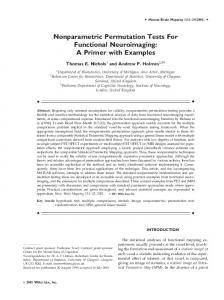
Figure 2: For our analysis of the Table 1 data, we generated 1000 resamples for the permutation test and computed each of 5 test statistics for each resample. Here is the scatterplot matrix showing the relationships between pairs of the 5 test statistics. Note the strong correlations between LTE and Beta, between M and GK, and the weaker correlation between LT and LTE or Beta.

Permutation Tests in Primatology

31

Table 3: P -values for permutation tests on infant handling data for baboons, using test statistics described in Section 3.2. All = All interactions = Table 1; Pass = Passive interactions = Table A.1; Un = Unsuccessful interactions = Table A.2; Succ = Successful interactions = Table A.3. The last row (in parenthesis) gives P -values from applying Mantel’s test to the 3-by-3 table and assuming approximate normality. Data Set Test Stat LTE LT M GK Beta (M)

PA

Pass

Un

Succ

0.010 0.044 0.000 0.001 0.004 (2.8e-007

0.009 0.060 0.003 0.011 0.004 0.008

0.016 0.089 0.003 0.002 0.000 0.0013

0.361 0.027 0.001 0.001 0.415 0.0014)

Table 4: Successful interactions by Infant Rank and Handler Rank (A); column percentages (B); adjusted residuals (C). These figures lend strong support to RH2. Handler’s rank

Infant Rank

Hi Mid Low

Hi

Mid

Low

Hi

0 19 3 (A)

3 6 14

2 22 43

0.0% 86.4% 13.6% (B)

Mid

Low

Hi

Mid

Low

13.0% 26.1% 60.9%

3.0% 32.8% 64.2%

−1.13 4.73 −5.93 (C)

2.22 −1.73 1.11

−0.65 −1.70 2.75

3.3 Significance tests on baboons data Using the scheme outlined in section 3.1 combined with the 5 test statistics, we perform permutation tests on the Table 1 data as well as on the data corresponding to the 3 categories of interactions Passive, Unsuccessful, and Successful (Tables A.1, A.2, and A3 in the Appendix). Table 3 summarizes the results. What jumps out of the table is that most p-values are small. The interest lies in the nuances. First note the clustering of test statistics by the similarity of results they give: LTE and Beta give similar results (small p-values, except for the large p-values with Successful); M and GK give similar results, and LT forms a cluster of one. These clusters are even clearer in the scatterplot matrix (Figure 2) of the 5 sampling distributions created by the 1000 resamples of the permutation test. Table 4 shows a breakdown for Successful interactions. Just looking at (A), we see that the strikingly large counts reside in precisely the cells — (Mid,High), (Low,Mid), and (Low,Low) — predicted by RH2. Tables 4(B) and 4(C) confirm

32

Thomas L. Moore and Vicki Bentley-Condit

this observation. These observations seem very consistent with a p-value of .027, which we obtain with the LT statistic for successful interactions. Table 5 gives adjusted residuals, p-values using the LT statistic, and total sample sizes for all 3 types of interaction. Looking first at just the adjusted residuals, we see evidence for RH2 for all 3 types of interactions, but with seemingly strongest evidence for Successful. The p-values sharpen this evidence: the .027 is the smallest p-value among the LT p-values, even though it is associated with the smallest sample size. Table 5: Adjusted residuals for Passive, Unsuccessful, and Successful interactions. P -values refer to the LT statistic; n’s are total counts for each table. Passive

Hi Mid Low

Unsuccessful

Successful

Hi

Mid

Low

Hi

Mid

Low

Hi

Mid

Low

3.04 2.32 −3.30

−1.13 −0.46 0.82

−1.23 −1.33 1.73

−0.68 2.98 −2.89

1.38 −0.76 0.55

−0.71 −2.11 2.23

−1.13 4.73 −5.93

2.22 −1.73 1.11

−0.65 −1.70 2.75

p = .060; n = 377

p = .089; n = 189

p = .027; n = 112

To summarize, LTE and Beta suggest RH1 holds for all types of interactions except Successful while LT suggests that RH2 does hold for Successful interactions. This analysis gives early evidence that LTE and LT distinguish between RH1 and RH2 for data tables such as ours. 3.4 Interpretation of results for baboon behavior From section 3.3 we can draw two conclusions regarding our test statistics: (1) The test statistics fall into two, inter-correlated clusters. LTE, LT, and Beta form one highly correlated cluster, while M and GK form a second cluster, uncorrelated with the first. (2) Within the LTE-LT- Beta cluster, LTE and Beta seem more similar than either is with LT and, moreover, there is an indication that LTE (and Beta) and LT distinguish well between hypotheses RH1 and RH2, an observation which is comforting given that LTE and LT were defined on intuitive grounds to make this very distinction. We will learn in section 4 that LTE and LT also have good power properties relative to RH1 and RH2, which leads us here to concentrate on interpreting the results for LTE and LT with regard to infant handling behavior in female baboons. To the primatologist, the results in Tables 3, 4, and 5 paint a very good picture of the intricacies of female baboon society. As background information for the reader who may not be versed in primatology, we note that dominance rankings are important forces within the females of the troop. High dominance translates

Permutation Tests in Primatology

33

into a variety of significant perquisites, such as access to preferred locations (e.g., shady spots on hot days), first access to food, choice of mates, and reproducing at a younger age. Moreover, the high-mid-low categories were fairly sharp in this troop. It is also known that at work in infant handling behavior are the following opposing forces: (1) The higher-ranked female handler in such behavior can use the interaction for her own satisfaction, i.e., the satisfaction of interacting with an “attractive” infant or she can use the interaction as a way of asserting her dominance over a lower ranked female. That is, there are nice and notnice reasons a handler attempts to handle. (2) A lower-ranked mother can use her infant to manipulate her position within the troop. By currying favor with higher ranked females in allowing the handling of her infant, she can befriend or ingratiate herself with the higher ranked female and in so doing reap some of the benefits of the higher rank; this phenomenon is called “status striving.” In essence, an infant is social capital. We say these forces work in opposition because there is risk of danger to the infant in infant handling. Interactions sometimes lead to injury or death, and this risk tends to be greater as the disparity between handler and mother dominance rank gets greater. With this background in mind, we can give some plausible interpretation to the patterns seen above. As a high-ranked female, you have little to lose in attempting to handle the infant of every female ranked lower than yourself. Attempting to handle above your rank is risky because a female who dominates you could make your life miserable. So you attempt lots of handling of lower ranked infants, hence the .009 and .016 p-values for Passive and Unsuccessful interactions, but the LTE p-value of .361 suggests you cannot count on being successful. So, every time the dominant female sits down within arm’s length of you and your infant (1 meter defines Passive interactions) you stay only as long as is necessary and then you leave. Alternatively, you see that she is making a move to grab your infant and you turn your back on her, resulting in an unsuccessful attempt. This cautious, cagy behavior from a mother is more pronounced toward females far above her rank, but the mother is more willing to allow the just-immediately-higher ranked female to be successful. This represents a less dangerous opportunity for status striving and is reflected in the more highly successful LT p-value of .027. Thus the significance tests reflect the complexities of female baboon society, one where the causes cannot be solely attributed to dominant handlers having their way, but rather where there are conflicting forces at work between a dominant female’s desire to handle an infant and the subordinate female’s need to curry favor through her infant while simultaneously protecting it.

34

Thomas L. Moore and Vicki Bentley-Condit

4. Power Study We now describe results of a computer simulation study we did to compare the power of our 5 test statistics vis a vis the two research hypotheses, RH1 and RH2. We ran our simulation study using S-Plus 7.0 for Windows using an HP laptop computer running Windows XP. Our simulation should be viewed as something of a pilot study in that we seek basic comparative power information among the proposed test statistics over a range of data production situations that is wide enough to give a sense of the robustness of the comparisons while still staying within the modest computational limits of S-Plus programming and the authors’ programming expertise. The results of our study suggest strongly that LTE and LT are valid choices for test statistics, which suffices for the purposes of the baboon application at hand. We defined a variety of situations in which data such as ours could arise and compared the power of the 5 test statistics at each situation. The results of these comparisons should guide us in choosing good test statistics when analyzing future data sets. To define a situation, we identified 7 factors that we could vary on a data table such as given by Table 1. Table A.4 summarizes these 7 factors, each of which was considered at two possible levels, designated conventionally as the “low value” and “high value.” Each combination of the 7 factors defines a situation. Each situation defines a possible state of nature that is consistent with either Research Hypothesis I or Research Hypothesis II. For a given situation, we randomly generated a set number of data tables. This set number we denoted by reps. We set reps at 200. For each of the 200 (reps) data sets for a given situation, we tested the null hypothesis using each of the 5 test statistics in a modified permutation test that used 100 random permutations. (Using each data set for all 5 test statistics provided some variance reduction for the comparisons.) This number of random permutations we designated by the variable resamples. While 200 reps and 100 resamples were small enough to allow practical run-times for our S-Plus simulations, they were also large enough to let us make useful distinctions between the test statistics. We used an α level of α = .05 for the simulations. Thus for each data set generated, we rejected the null hypothesis whenever the associated empirical pvalue (using 100 resamples) was .05 or less. If X of the 200 random data sets for a given situation resulted in a statistically significant result then the estimated power for that combination of test statistic and situation was X/200. A randomly generated data set will be a matrix of counts as in Table 1. Columns will correspond to female handlers and rows to infants. For each situation considered, we generated such a random data set using a product multinomial

Permutation Tests in Primatology

35

distribution. Here is how that process works. Factor 1 is n, the total sample size for our data table. In Table 1, n = 678 but in our power study we allowed n to be either 48 or 96. Factor 2 is the table’s dimensions. For Table 1 the dimensions were 11 by 23, but for the simulation we considered values of 6 by 12 or 12 by 24. Factor 3, res, stands for which of the two research hypothesis we wish to simulate; it’s values are Research Hypothesis I (RH1) or Research Hypothesis II (RH2). Factor 4, magn, stands for the magnitude of the difference between the null hypothesis and the research hypothesis (RH1 or RH2) that is under consideration. This magnitude is a ratio of probabilities. To be specific, for a given research hypothesis (RH) and a given handler, RH predicts that infants of certain ranks are more likely to be handled by that handler than are other infants. These infants predicted more likely to be handled will be called consistent (C); the others will be called inconsistent (I). For example, for RH1, infants of rank less than or equal to the handler’s rank are consistent. The factor magn stands for the ratio pC |pI where pC stands for the probability she handles any particular consistent infant and pI stands for the probability she handles any particular inconsistent infant. So, for example, with RH1 and magn=3.0, the probability a given handler will handle a particular infant at or below her own rank is 3 times the probability she will handle a particular infant who is above her in rank. Factors 5 and 6, rowranks and colranks, represent the distribution of high (1), mid (2), and low (3) ranks for infants and handlers, respectively. For Table 1, rowranks=(1, 2, 2, 2, 2, 3, 3, 3, 3, 3, 3) and colranks=(1, 1, 1, 1, 2, 2, 2, 2, 2, 2, 2, 3, 3, 3, 3, 3, 3, 3, 3, 3, 3, 3, 3). The low values for either rowranks or colranks are a uniform distribution. For example, if the table is 6-by-12 the low value for rowranks is (1,1,2,2,3,3) and colranks is (1,1,1,1,2,2,2,2,3,3,3,3). High value for a row or column dimension of 6 is (1,2,2,3,3,3), for 12 is (1,1,2,2,2,2,3,3,3,3,3,3), and for 24 is (1,1,1,1,2,2,2,2,2,2,2,2,3,3,3,3,3,3,3,3,3,3,3,3). Finally, Factor 7, enz, represents a vector of sample sizes for the productmulitnomial distribution. The length of enz is equal to the number of handlers dictated by the particular situation, that is by the number of columns in the random data set being produced. The low value of enz puts a uniform set of sample sizes for each of the handlers. For example, when there are 12 handlers (the 6-by-12 case) and the total sample size is 96 (n = 96), the sample sizes for the multinomial distribution are 8, 8, . . . , 8. At the high value, we use a nonuniform or ‘ragged’ set of sample sizes. When there are 12 columns (or handlers) the multinomial sample sizes are 6 2 6 2 6 2 6 2 6 2 6 2 for n = 48 or double this vector for n = 96. When there are 24 columns the sample sizes are 3 1 3 1 3 1 3 1 3 1 3 1 3 1 3 1 3 1 3 1 3 1 3 1 for n = 48 or double this for n = 96. Now, for a combination of the 7 factors, the following process will produce a

36

Thomas L. Moore and Vicki Bentley-Condit

random data set: • A given handler determines a column of counts in the random data set, call it column j; • She generates enzj counts from a multinomial distribution; • The probabilities for her multinomial distribution are determined by magn; • That is, the probability she interacts with any consistent infant is magn times the probability she interacts with any given inconsistent infant. The collection of counts generated by this set of independent multinomial counts for each handler forms the final random product-multinomial random data set. We chose to run a 2∧ (7 − 3) design, or 16 runs, which is a resolution IV design that allowed us un-confounded estimates of all 7 main effects. That is, the main effects could be estimated free of the two-way interactions. Given the limitations of an S-Plus programming environment, this design gave a reasonable range of situations while allowing us to use reasonable values of both reps and resamples. Our choices of factors and factor levels were intuitive, based on the desire to span a range of practically useful situations and to also pick levels that would let us make distinctions among the test statistics. We used sample sizes much smaller than encountered in the actual study (48 and 96 versus as large as 678 in the full Table 1) based upon a few small runs that suggested that with large sample sizes powers could be so large as to make comparisons difficult. The design matrix along with power estimates at each combination for each test statistic is given in Table A.5. Table A.6 in the Appendix shows the results of an analysis of the main effects for the 7 factors, which provides a gauge on our choices of factor levels. Tables A.6A, A.6B, and A.6C give respectively the estimated main effects, their standard errors, and their z-scores. Almost all main effects are significant, suggesting that we chose factor levels that spanned a wide enough collection of situations to be able to see power differences between the test statistics. The ultimate goal of a power study was to compare power across the five test statistics over the various situations. Table 6 summarizes comparisons between test statistics for each of the 16 situations. To make these comparisons, we computed a standard error for the difference between the powers of 2 different test statistics. To compute this standard error we used the formula Var (ˆ p1 − pˆ2 ) = Var (ˆ p1 )+ Var (ˆ p2 ) − 2 Cov (ˆ p1 , pˆ2 ), where pˆ1 and pˆ2 stand for power estimates (i.e., sample proportions) for some two test statistics at some situation. Table 6 summarizes the results. The “comments” column summarizes the pairwise comparisons between all pairs of test statistics for each situation. For

Permutation Tests in Primatology

37

these comparsions we used a liberal definition of statistical significance, namely α = .05 in a one-sided test. Table 6: The estimated powers for each of the 5 test statistics at each of the 16 factor combinations given in Table A.5 using 200 reps per situation and 100 resamples in each permutation test. The RH? column tells which research hypothesis (RH1 or RH2) is modeled by that situation. The Comments column indicates which test statistics outperform which other test statistics. The > symbol indicates “statistically better than;” the ∼ symbol indicates not significantly better than. The test statistics are abbreviated in the comments column. We use the > symbol if the difference exceeds 1.645 standard errors, which corresponds to a .05-level, one-sided criterion. Non-transitivities may occur, which accounts for multiple comments in some cases. When test statistics are not statistically different, the one with the larger estimate is listed to the left. 1 2 3 4 5 6 7 8 9 10 11 12 13 14 15 16

LTE 0.230 0.420 0.180 0.355 0.095 0.250 0.250 0.335 0.765 0.860 0.930 0.965 0.660 0.855 0.625 0.960

LT 0.150 0.225 0.190 0.270 0.315 0.530 0.345 0.605 0.505 0.660 0.745 0.645 0.975 1.000 0.980 1.000

M 0.155 0.140 0.130 0.145 0.095 0.295 0.205 0.225 0.315 0.635 0.365 0.645 0.710 0.310 0.440 0.755

GK 0.170 0.170 0.140 0.160 0.095 0.375 0.195 0.240 0.425 0.650 0.445 0.720 0.825 0.400 0.505 0.800

Beta RH? Comments 0.205 1 LTE ∼ Beta > LT; LTE > GK ∼ M; all others ∼ 0.375 1 LTE ∼ Beta > LT,GK,M; LT ∼ GK > M 0.160 1 LT ∼ LTE ∼ Beta; LT > GK∼M; LTE > M; others ∼ 0.155 1 LTE > LT > GK,Beta,M; others ∼ 0.045 2 LT > LTE,M,GK > Beta; others ∼ 0.240 2 LT > GK > M,LTE,Beta; others ∼ 0.285 2 LT > Beta,LTE,M,GK; Beta>M,GK; LTE>GK;others ∼ 0.385 2 LT > Beta∼LTE > GK∼M 0.480 1 LTE > LT∼ Beta,GK,M; LT > GK > M; Beta > M 0.340 1 LTE > LT,GK,M,Beta; LT∼GK∼M > Beta 0.735 1 LTE > LT,Beta,GK,M; LT∼Beta > GK > M 0.920 1 LTE > Beta > GK > LT ∼ M 0.810 2 LT > GK,Beta,M,LTE; GK∼Beta > M∼LTE 0.855 2 LT > LTE,Beta,GK,M; LTE∼Beta > GK > M 0.685 2 LT > Beta > LTE > GK > M 0.925 2 LT > LTE > Beta > GK > M

Conclusions regarding the test statistics: A primary message coming from Table 6 is that the LTE or LT statistics perform as well as or better than the other 3 test statistics. Moreover, in all but one situation (the third one) LTE is best when the given situation models RH1 and LT is best when the situation models RH2. For situations 4 through 16, this summary is clean, in that LTE or LT is not only the highest estimated power, but it is statistically superior to the other 4. In situation 3, LT and LTE are reversed regarding estimated power, but the difference is not statistically significant. In situations 1, 2, and 3 the Beta statistic is not statistically inferior to LTE (or LT in situation 3), but it is inferior in absolute terms. Since Beta is much harder to compute than the LTE or LT statistics, one would not favor it unless it had proved to be statistically superior. Thus, the take-away message is that LTE and LT are good test statistics for testing for our two research hypotheses in the female handing data.

38

Thomas L. Moore and Vicki Bentley-Condit

0.76 0.72 0.68

LTE.rem.inf.Pass

LTE vs. Removed Infant ID (Passive)

2

4

6

8

10

ID

0.06 0.02

p.rem.inf.Pass.LTE

0.10

p-value with LTE vs. Removed Infant ID (Passive)

2

4

6

8

10

ID

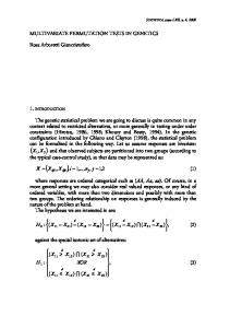
Figure 3: Gives 2 plots from remove-one-infant sensitivity analysis. The top plot is an example of stability. The bottom plot is one of instability.

5. Sensitivity Analysis Lunneborg (2000, pp. 309-318) introduces the notion of “stability of description” for permutation tests applied to an observational study. In particular, he argues (p. 311) that “... a fair description is one that is stable, that is, one that is relatively uninfluenced by the presence or absence of specific cases.” He applies this notion (Lunneborg 2002) to our data by considering the stability of the LTE test statistic under a remove-one-at-a-time strategy. There (p. 14) he asserts, “... it is important to verify that the summary statistic in a nonrandomized study fairly reflects the whole of the data, and, in particular, that it is not unduly influenced by the inclusion in the study of one particular source of observations.” He then shows that the LTE test statistic is stable on removal of one female handler at a time and also on removal of one infant at a time, when looking at the data in Table 1. Here we extend Lunneborg’s results in two ways, by: (a) looking at stability with respect to each of LTE and LT for each category of interaction: Passive, Unsuccessful, and Successful; and (b) looking at stability (again for both LTE and LT and for each category of interaction) with respect to the null model analysis, i.e., by using p-value as our descriptive statistic. For the null model analysis, we use the same 1000 resamples as in the original analysis. First, instead of LTE as defined heretofore, we will use a normalized version of LTE that takes LTE divided by the total number of interactions in the table. Lunneborg (2002, pp. 14-15) suggests this variant as a way of meaningfully

Permutation Tests in Primatology

39

making it possible to compare LTE values between two tables with differing total counts, but which for any given table leads to exactly the same p-value since it is a scaled version of the raw LTE statistic. The interpretation of the normalized LTE is that it represents a difference in the proportion of consistent interactions and the proportion of inconsistent interactions. Figure 3 gives two plots exhibiting one situation of stability (on top) and one of instability (on the bottom). The stable plot on the top shows LTE values versus Infant ID. Note the fairly uniform distribution of LTE value, so that no particular infant exerts undue influence on the LTE value for Passive interactions. The normalized LTE value for Passive interactions for the full table is 0.719 = 271/377. Notice that in the stable graph, there is a fairly uniform distribution of LTE values about .719, ranging from about .67 to about .79. Contrast this to the plot on the bottom, which shows p-values from a null model analysis against removal of one infant at a time. Table A.7 shows the remove-one-infant summary for the two test statistics, LTE and LT, and the 4 data tables: All, Passive, Unsuccessful, and Successful. Table A.8 shows the remove-one-infant summary for the null model analysis (i.e., p-values). The results in Table A.7 show general stability of the original analysis. Table A.8 exhibits only a very slight instability: the removal of infant 1 for Passive interactions causes a p-value increase from values between .01 to .03 to a p-value with infant 1 removed of .104. While the .104 value is an outlier, it is still not such an alarmingly high p-value to completely discredit the original analysis that gave evidence for RH1 for Passive interactions. In similar fashion, we studied stability of the original analysis using a removeone-handler-at-a-time strategy. When one removes a handler, one also removes that handler’s infant in cases where she is a mother. This makes sense because our procedure does not know how to permute ranks when the infant has no mother. Then one describes the reduced data table, again using either the test statistic as a summary value or the p-value as as summary value. Tables A.9 and A.10 give the results of this stability analysis. By plotting these values, one can see that removing handler #1 (the mother of infant #1) causes a similar slight instability in p-value results. Otherwise, the results are all very stable. Summarizing our stability analysis, we conclude that infant #1 and its mother, handler #1, exert a modest influence on the null model results. This may not be surprising, given that handler #1 was one of only 4 high-ranked females and was the only one with an infant. Still, the level of instability is not high, so the original conclusions are compromised modestly, at most.

40

Thomas L. Moore and Vicki Bentley-Condit

6. Conclusions In this paper, we describe the use of permutation tests to analyze a twoway table where counts “enter” the table in clusters, invalidating a traditional chi-square-like analysis. Whereas previous researchers have coerced statistical inference into a chi-square situation by means of an either-or approach for each cell (where 1’s represent any non-zero count), permutation tests allow for a legitimate use of all the data. We define simple test statistics, LTE and LT, tailored intuitively to be sensitive to two versions of the research hypothesis that females tend to handle down the dominance hierarchy. We apply these tests to an overall table of interactions (mostly to illustrate the method) and then separately to the three separate types of interactions – Passive, Unsuccessful, and Successful – that make up the overall table. We interpret the results of this to support a nuanced view of how infant handling behavior by adult females occurs within this troop of baboons, in particular, how there are forces causing more dominant females to handle down the hierarchy and subordinate females to want to curry favor up the hierarchy through their infants while also wanting to keep their infants free from unsafe handling by much higher ranked females. Through a power analysis, we show that our test statistics outperform other test statistics regarding the two research hypotheses and, finally, we show that the results of our data analysis are fairly stable to removing infants or handlers one at a time. Acknowledgements The authors thank Tom Loughin, George Cobb, David S. Moore, Gary Oehlert, and Emily Moore for their invaluable help and support on this project, and thank Avram Lyon and Karen Thomson for technical assistance. Research supported in part by the Frank and Roberta Furbush Scholar Fund at Grinnell College. References

Agresti, A. (2002). Categorical Data Analysis (2nd ed.), John Wiley. Bentley-Condit, V. K., Moore, T. L., and Smith, E. O. (2001). Infant handling by tana river adult female yellow baboons. (papio cynocephalus cynocephalu). American Journal of Primatology 55, 117-130. Dagosto, M. (1994). Testing positional behavior of malagasy lemurs: a randomization approach. American Journal of Physiological Anthropology 94, 189-202.

Permutation Tests in Primatology

41

de Waal, F. (1990). Do rhesus mothers suggest friends to their offspring? Primates 31, 597-600. Dow, M. and de Waal, F. (1989). Assignment methods for the analysis of network subgroup interactions. Social Networks 11, 237-255. Dwass, M. (1957). Modified randomization tests for nonparametric hypotheses. The Annals of Mathematical Statistics 28, 181-187. Gotelli, N. J. and Graves, G. R. (1996). Null Models in Ecology. Smithsonian Institution Press. Knox, K. and Sade, D. (1991). Social behavior of the emperor tamarin in captivity: components of agonistic display and agonistic network. International Journal of Primatology 12, 439-480. Loughin, T. M. (2002). Personal communication. Lunneborg, C. E. (2002). Infant Handling by Female Baboons: A Sensitivity Analysis. STATS 33, 13-15. Moore, T L. and Bentley-Condit, V. (2001). Using Permutation Tests to Study Infant Handling by Female Baboons. STATS 31, 7-14. Mundry, R. (1999). Testing Related Samples with Missing Values: A Permutation Approach. Animal Behavior 58, 1143-1153. Patefield, W. M. (1982). Exact Tests for Trends in Ordered Contingency Tables. Applied Statistics 31, 32-43. Small, M. F. (1990). Alloparental Behaviour in Barbary Macaques. Macca sylvanus, Animal Behavior 39, 297-306. Small, M. F. (2004). Personal communication. Thompson, L. A. (2002). S-Plus (and R) Manual to Accompany Agresti’s Categorical Data Analysis, (2nd ed.), on line at: https://home.comcast.net/˜lthompson221/#CDA. Received May 16, 2008; accepted July 13, 2008.

Thomas L. Moore Department of Mathematics and Statistics Grinnell College Grinnell, IA 50112, USA [email protected] Vicki Bentley-Condit Department of Anthropology Grinnell College Grinnell, IA 50112, USA [email protected]