Permutation Predictor Tests in Linear Regression

DOI: http://dx.doi.org/10.5351/CSAM.2013.20.2.147

Communications for Statistical Applications and Methods 2013, Vol. 20, No. 2, 147–155

Permutation Predictor Tests in Linear Regression Hye Min Ryua , Min Ah Woob , Kyungjin Lee c , Jae Keun Yoo 1,c a

Clinical Research Coordination Center, National Cancer Center b Korea Information and Communication Industry Institute c Department of Statistics, Ewha Womans University

Abstract To determine whether each coefficient is equal to zero or not, usual t-tests are a popular choice (among others) in linear regression to practitioners because all statistical packages provide the statistics and their corresponding p-values. Under smaller samples (especially with non-normal errors) the tests often fail to correctly detect statistical significance. We propose a permutation approach by adopting a sufficient dimension reduction methodology to overcome this deficit. Numerical studies confirm that the proposed method has potential advantages over the t-tests. In addition, data analysis is also presented.

Keywords: Linear regression, non-normality, permutation test, small samples.

1. Introduction Regression is a statistical methodology to study the conditional distribution of a response variable Y ∈ R1 given a set of predictors X ∈ R p = (X1 , . . . , X p )T . The regression seeks an investigation of how the response Y is changed given X. Subsequently, the following model-based regression (linear regression) is popular: Y | X = α + βT X + ε,

(1.1)

where β = (β1 , . . . , β p )T and ε∼N(0, σ2 ). In the model of (1.1), the vector of β represents unknown coefficients and measures the effects of predictors to the regression. For example, if βi = 0, the corresponding predictor Xi does not contribute to the regression. When numerous predictors are considered in the regression, there is a possibility that many unnecessary predictors are involved. Therefore it is best to select significantly important ones among all predictors to the regression because a regression model with smaller set of predictors may be easier to maintain as well as help to increase prediction accuracies. In regression, a procedure to select important predictors and to keep them alone is called variable selection. There exist many variable selection procedures in the context. We briefly explain the classical and most widely used ones in practice. The first one should be t-tests for testing H0 : βi = 0 for i = 1, . . . , p. The constructed test statistic is ti∗ = βˆi /se(βˆ i ), where βˆ i represents the ordinary least square (OLS) estimate of βi and se(βˆ i ) does the corresponding standard error. Then, the statistic ti∗ For the corresponding author Jae Keun Yoo, this work was supported by Basic Science Research Program through the National Research Foundation of Korea (KRF) funded by the Ministry of Education, Science and Technology (2012040077). 1 Corresponding author: Associate Professor, Department of Statistics, Ewha Womans University, 11-1 Daehyun-Dong Seodaemun-Gu, Seoul 120-750, Korea. E-mail: [email protected]

Hye Min Ryu, Min Ah Woo, Kyungjin Lee, Jae Keun Yoo

148

follows t distribution with (n − p − 1) degrees of freedom under the normality and constant variance of ε. For testing multiple coefficients equal to zeros and testing H0 : βi = β j = · · · = βk = 0 for i , j , · · · , k, general F-tests are often conducted. Let M1 stand for a current model and M0 do for a smaller model under the null hypothesis. Then the test statistic and its distribution are as follows: F∗ =

(SSE0 − SSE1 )/(d f0 − d f1 ) ∼ F(d f0 −d f1 ),d f1 , SSE1 /d f 1

where SSEm and d fm represent residual sums of squares and its degrees of freedom for model Mm , m = 0, 1, respectively. Another way is to use Akaike’s information criteria (AIC) and Schwarz’ Bayesian information criteria (BIC). The formulas for AIC and BIC are as follows: AIC = n log(SSE) − n log(n) + 2p and BIC = n log(SSE) − n log(n) + [log(n)]p. In both the cases, smaller values indicates more important predictors. The differences between AIC and BIC are placed on the third term. If n < 8, the term for AIC is larger than that for BIC. Therefore, the BIC tends to favor more parsimonious models according to Kuntner et al. (2005). The t or general F-tests and the information criteria have quite different aspects to select variables. The former can directly decide which predictors do have null effects to the regression as well as which one is the least important. In addition, contrast effects between predictors are easily tested. This is why the two tests are mostly preferred to usual non-statistical practitioners over the information criteria. However, the latter can provide evidence on which ones are the least important but they cannot properly conduct evaluations of contrast effects. Therefore, the information criteria are typically preferred in use for automatic search procedures for variable selection such as backward, forward, and stepwise selections. These popular ways for variable selection produce unreliable selection results under relatively smaller sample sizes than the number of parameters and non-normal error. False selections occur mainly due to type-II-error and the null hypothesis of H0 : βi = 0 is not often rejected (although the hypothesis is not true). Therefore, a set of selected predictors are usually smaller than the true one. To overcome this deficit, a permutation test is proposed by adopting sufficient dimension reduction. The sufficient dimension reduction is non-parametric and often works well in relatively smaller samples. The proposed permutation approach is expected to improve the problems of existing and popularly used methods discussed above; in addition, statisticians can easily use it and understand the results since the permutation approach provides p-values. The paper is organized as follows. In Section 2 we define predictor effect hypothesis and propose permutation predictor effect tests in linear regression. Section 3 is devoted for numerical studies and real data application. Finally we summarize our work in Section 4.

2. Permutation Predictor Tests 2.1. Predictor effect hypothesis Variable selection in a regression of Y ∈ R1 | X ∈ R p is defined as conditional independences of the response given predictors. To illustrate this, first, partition the original p-dimensional predictors X into (XH ∈ Rh , XH⊥ ∈ R(p−h) ). The subset XH have no effects to a regression of Y | X, if and only if the complement set of XH⊥ alone is fully informative to the regression. Equivalently, the conditional distribution of Y | X is equal to that of Y | XH⊥ , which can be equivalently rephrased as that Y is independent of X given XH⊥ . The arguments discussed above can be summarized as the following three equivalent statements: (a) the subset XH has no effects to a regression of Y | X; (b)

Permutation Predictor Tests in Linear Regression

149

FY | X (·) = FY | XH⊥ (·); (c) Y X | XH⊥ , where F(·) and stands for a cumulative probability function and statistical independence, respectively. Effects of predictors to regression can be evaluated as subsets of predictors as well as their contrasts. In this sense, variable selection is a special interest of predictor effects to regression. Therefore, we need to generalize variable selection to evaluate predictor effects. Let H, H, and PH represent an h-dimensional predictor subspace of X with h ≤ p, its p × h orthonormal basis matrix, and the orthogonal projection operator onto H with usual inner-product subspace, respectively. And, H⊥ ∈ R p×(p−h) stands for the orthonormal basis matrix for the orthogonal complement of H. Then the effects of predictors are defined as the following equivalent statements: (a1) PH X has no effects to regression of Y | X; (b1) FY|X (·) = FY|PH⊥ X (·); (c1) Y X | PH⊥ X, where PH + PH⊥ = I p . Hereafter, any of the three statements given in (a1), (b1), and (c1) will be called predictor effect hypothesis. Let us illustrate the hypothesis. If one selects H as the ith p-dimensional canonical basis vector, ei with the ith element equal to one and zeros elsewhere, PH X is equal to Xi in order to evaluate whether or not Xi is significantly important to regression. If one chooses H = (0.5, −.25, −0.25, 0, . . . , 0)T , it is to determine whether or not the effect of X1 is equal to the average of the effects of X2 and X3 . The former example is a case of variable selection and the latter is of the contrasts.

2.2. Permutation predictor effect tests in linear regression Under linear regression, effects of each predictor are measured by the corresponding regression coefficients. So, the non-parametric statements of predictor effect hypotheses are evaluated through the regression coefficients and we can formulate the evaluation as a procedure of parametric hypothesis tests. Under linear regression in (1.1), PH X has no effects to regression of Y | X, if and only if PH β = 0, equally HT β = 0. Therefore, the effect of PH X is easily evaluated through testing the hypotheses of H0 : HT β = 0 versus H1 : HT β , 0. Hereafter, for notational conveniences, we define that XH = PH X and XH⊥ = PH⊥ X. Popular t-tests allow us to conduct these hypothesis tests easily, but they have limits in use under relatively smaller samples and non-normal errors. The conditional statement (c1) in Section 2.1 has the same form as the key statement used in sufficient dimension reduction (SDR). Its main idea is to replace the original p-dimensional predictor X by lower-dimensional linearly-transformed predictors ηT X with η ∈ R p×m and m < p such that Y

X | ηT X.

(2.1)

The minimal subspace among all possible subspaces spanned by the columns of η satisfying (2.1) and its dimension are called the central subspace and the structural dimension. For more about sufficient dimension reduction, readers can refer Cook (1998). The same representation of (c1) and (2.1) offer a possibility to adopt methodologies used in SDR. Here we use a permutation approach to test the null hypothesis of HT β = 0. The permutation tests in SDR were suggested in Cook and Weisberg (1991) and formalized in Yin and Cook (2002) to estimate the structural dimension. However, predictor effect hypotheses must be tested here and do not have a direct application to our case. The key part in the permutation test procedure proposed by Yin and Cook (2002) is to permute ηˆ T⊥ X to generate permuted samples, where the p × (p − m) matrix ηˆ ⊥ is the orthonormal complement matrix of ηˆ ∈ R p×m such that ηˆ T⊥ ηˆ ⊥ = I(p−m) and ηˆ T⊥ ηˆ = 0. Therefore, we have to find appropriate objects randomly permuted for adapting the permutation tests into our problem. For this, based on the

Hye Min Ryu, Min Ah Woo, Kyungjin Lee, Jae Keun Yoo

150

null hypothesis of HT X, the original predictor X is partitioned into (XH = HT X, XH⊥ = HT⊥ X). Then, since Y X | HT⊥ X under the null hypothesis, we can randomly permute XH . We will denote permuted perm samples of X as Xperm = (XH , XH⊥ ). Next, to conduct predictor effect tests through the random permutations, we need to define a statistic to evaluate whether or not HT β = 0. For this we think of the following reasoning. If the null hypothesis is true, we expect that the distances between two vectors of βˆ and βˆ H = PH⊥ βˆ must be relatively close. After normalizing βˆ and βˆ H to have unit length, the following distance is measured between the two: ( ) ˆ λˆ H = 1 − βˆ T βˆ H βˆ TH β. (2.2) To understand λˆ H , we consider two extreme cases. The first extreme case is that β = βH . That is, a subspace spanned by β is equivalent to a subspace of the orthogonal complement of H. If so, the value of βT (βH βTH )β after normalization is equal to one, and hence the value of 1 − βT (βH βTH )β becomes zero. The second extreme case is β = PH β. A subspace spanned by β is a subspace of of H. Then, we have βT (βH βTH )β = 0, and hence the value of 1 − βT (βH βTH )β is equal to one. From the two extreme cases, λˆ H should vary from zero and one. The first extreme case holds, if the null hypothesis is true. So relatively smaller values of λˆ H or ones close to zero imply that the null hypothesis is true. However, if λˆ H is relatively larger or close to one, then the null hypothesis is indicated to be false. Here λˆ H in (2.2) is proposed as a statistic to test H0 : HT β = 0. We compute λˆ H from the original ˆ perm sample and permuted samples that will be respectively denoted as λˆ ref H and λH . Then an empirical ˆ perm computed from each permuted sample. Finally, sampling distribution of λˆ ref H is constructed by λH perm T p-values to test H0 : H β = 0 are calculated as the percentages of λˆ H > λˆ ref H . We summarize the procedure as follows: Algorithm of permutation predictor tests 1. Obtain the OLS estimate βˆ of β from the original sample of Y and X. 2. Based on H0 : HT β = 0, partition X into (XH = HT X, XH⊥ = HT⊥ X) with HT⊥ H = 0. 3. Compute βˆ H = PH⊥ βˆ and normalize βˆ and βˆ H . Then calculate λˆ ref H . perm

4. Permute XH randomly and construct permuted predictors of Xperm = (XH , XH⊥ ). 5. Obtain the OLS estimate βˆ perm from the permuted samples of Y and Xperm . perm

6. Compute βˆ H

perm

perm

= PH⊥ βˆ perm and normalize βˆ perm and βˆ H . Then calculate λˆ H .

7. Repeat steps 4 to 6 K times. 8. Calculate the percentages of λˆ perm > λˆ ref among all λˆ perm s, and report the percentages as p-values for testing H0 : HT β = 0.

3. Simulation Studies and Data Analysis 3.1. Simulation studies For all numerical studies, five dimensional predictors X = (X1 , . . . , X5 )T were generated from multivariate normal distributions with mean 0 and the correlation matrix Σ, whose diagonal and offdiagonal elements are (respectively) equal to one and ρ for ρ = 0.3, 0, 5, 0.7.

Permutation Predictor Tests in Linear Regression

151

The following artificial model was constructed: Y | X = X1 + X2 + 0.5X3 + ε, where an random error ε is distributed as one of the three distributions of standard normal distribution, χ2 distributions with two degrees of freedom, and t distributions of three degrees of freedom. In addition we considered 15, 30, 50 and 100 sample sizes and the model was iterated 500 times. By construction, the model has the following values for the regression coefficients: β1 = β2 = 1;

β3 = 0.5;

β4 = β5 = 0.

For this model, we tested the following seven hypothesis: H0 : βi = 0 H0 : β1 = β2

versus versus

H1 : βi , 0, i = 1, . . . , 5; H1 : β1 , β2 ;

H0 : β2 = β3

versus

H1 : β2 , β3 .

For i = 1, 2, 3, the null hypothesis of βi = 0 is false, while it is true for i = 4, 5. Also, the null hypothesis of β1 = β2 is true, but that of β2 = β3 is false. To report the numerical studies, the percentages of the rejections of each null hypothesis were computed with level 5%. Therefore, in the case that the null hypotheses are true, the rejection percentages indicates the observed levels, and the tests are more desirable, if the percentages are close to 5%, which is the nominal level. However, if the null hypotheses are false, the rejection percentages represent the observed powers and the tests become more powerful as they are closer to 100%. To test H0 : βi = 0, we used usual t-tests in linear regression and the proposed permutation tests for H = ei ∈ R5 , i = 1, . . . , 5. As results, we report the rejection percentages of H0 : β3 = 0 and H0 : β4 = 0, because the asymptotic behaviors of testing H0 : βi = 0 for i = 1, 2 by the proposed permutation tests and t-tests are similar to those of H0 : β3 = 0. Omitting the results for H0 : β5 = 0 is the same reason. Tables 1–3 summarize these results. In addition, the permutation tests for H = (1, −1, 0, 0, 0)T and H = (0, 1, −1, 0, 0)T and general F-tests were conducted to test H0 : β1 = β2 and H0 : β2 = β3 . We summarize these numerical studies in Table 4 and Table 6. Tables 1–3 represent the characteristic patterns observed in other simulations. Regardless of distributions of random errors and correlation among the predictors, the proposed permutation tests are more powerful than usual t-tests. Also the power estimations in usual t-tests are greatly affected, especially with smaller samples, by the distributions of the random errors, while they are not in the permutation tests. Overall, with smaller samples, the proposed permutation tests clearly outperforms the t-tests, and reaches 100% faster than the t-tests. The permutation tests are affected by the correlation among the predictors so that their higher correlations make the observed levels worse, while usual t-tests are consistent to the correlation in the estimation of the nominal level. In the permutation samples, effects of unimportant predictors tend to be overestimated, and this can be partial reason that the permutation tests have larger observed levels than actual levels. From the simulation, we learn that the permutation tests often tend to reject the hypothesis of βi = 0. This implies that the permutation tests would keep more variables than usual t-tests in practice. With smaller samples, this should be a good property, in sense that it provides strong evidence that the corresponding predictors are not important, if the tests do not reject H0 : βi = 0, i = 1, . . . , p. According to Tables 4–6, there are no notable differences between the permutation tests and general F-tests in the estimations of level and power.

Hye Min Ryu, Min Ah Woo, Kyungjin Lee, Jae Keun Yoo

152

Table 1: Percentages of rejection of H0 : βi = 0 for i = 3, 4 with ε ∼ N(0, 1); Perm: permutation tests; t: t-test

n = 15 n = 30 n = 50 n = 100

ρ = 0.3 β3 = 0 β4 = 0 Perm t Perm t 40.0 31.0 10.0 3.0 65.0 53.0 8.0 7.0 84.0 77.0 6.0 5.0 100 100 5.0 7.0

ρ = 0.5 β3 = 0 β4 = 0 Perm t Perm t 50.0 24.0 10.0 2.0 66.0 40.0 11.0 5.0 87.0 74.0 9.0 3.0 100 96.0 8.2 4.0

ρ = 0.7 β3 = 0 β4 = 0 Perm t Perm t 53.0 15.0 29.0 6.0 71.0 34.0 21.0 6.0 78.0 50.0 20.0 6.0 98.0 80.0 17.0 4.0

Table 2: Percentages of rejection of H0 : βi = 0 for i = 3, 4 with ε ∼ χ21 ; Perm: permutation tests; t: t-test

n = 15 n = 30 n = 50 n = 100

ρ = 0.3 β3 = 0 β4 = 0 Perm t Perm t 31.0 25.0 12.0 3.0 56.0 41.0 6.0 7.0 66.0 51.0 6.0 5.0 94.0 92.0 7.0 4.0

ρ = 0.5 β3 = 0 β4 = 0 Perm t Perm t 46.0 21.0 17.0 5.0 59.0 33.0 19.0 7.0 65.0 40.0 12.0 3.0 89.0 82.0 11.0 7.0

ρ = 0.7 β3 = 0 β4 = 0 Perm t Perm t 44.0 12.0 36.0 4.0 64.0 24.0 26.0 6.0 64.0 23.0 25.0 5.0 82.0 52.0 17.0 5.0

Table 3: Percentages of rejection of H0 : βi = 0 for i = 3, 4 with ε ∼ t3 ; Perm: permutation tests; t: t-test

n = 15 n = 30 n = 50 n = 100

ρ = 0.3 β3 = 0 β4 = 0 Perm t Perm t 29.0 17.0 9.0 6.0 40.0 24.0 7.0 3.0 64.0 45.0 7.0 5.0 84.0 73.0 6.0 5.0

ρ = 0.5 β3 = 0 β4 = 0 Perm t Perm t 22.0 5.0 17.0 1.0 45.0 24.0 13.0 4.0 60.0 40.0 10.0 4.0 82.0 67.0 9.0 2.0

ρ = 0.7 β3 = 0 β4 = 0 Perm t Perm t 38.0 9.0 27.0 7.0 44.0 11.0 23.0 4.0 60.0 27.0 22.0 4.0 78.0 52.0 17.0 2.0

In the coordinate tests, the permutation tests and the t-tests produced quite different results, while the permutation tests and general F-tests were similar in the contrast tests. The reason why both the approaches produced similar results for the contrast tests in linear regression can be thought of as follows. For the coordinate effect tests, both the test statistics can be computed from one OLS fit computed under the alternative hypothesis, although it can be computed from the fits under the null and alternative hypotheses for usual t-tests. However, the two tests use the same information, so permutation tests yield more desirable results. However, for the contrast tests general F-tests should use information acquired from the two fits under the null and alternative hypotheses, while the permutation tests have to use information only under the alternative hypothesis. Usage of the supplemental information obtained from the null hypothesis in general F-tests is a possible reason why the permutation tests and general F-tests showed similar results in numerical studies.

3.2. Data analysis In this section, the proposed method is applied to a cloud seeding data introduced in Cook and Weisberg (1999, p.313). The data was collected to judge the success or failure of cloud seeding designed to increase rainfall. The original data contains seven variables; action (A) with 1 if seeded, or 0 otherwise; a time trend; the suitability (S ) for seeding score; cloud over in the experimental area; prewetness (P); echo motion category with 1 or 2, a measure of the type of clouds present; rainfall (R) in the target area following action. For illustration purpose, we consider the following regression: E{log R | (A, S , P)} = α + β1 A + β2 log P + β3 S + β4 AS + β5 A log P.

(3.1)

Permutation Predictor Tests in Linear Regression

153

Table 4: Percentages of rejections of H0 : β1 = β2 and H0 : β2 = β3 with ε ∼ N(0, 1); Perm:permutation tests; t:t-test

n = 15 n = 30 n = 50 n = 100

β1 = β2 Perm GF 9.0 8.0 6.0 4.0 3.0 2.0 5.0 5.0

ρ = 0.3

β2 = β3 Perm GF 10.0 7.0 35.0 31.0 49.0 52.0 79.0 79.0

β1 = β2 Perm GF 3.0 3.0 5.0 6.0 8.0 9.0 5.0 8.0

ρ = 0.5

β2 = β3 Perm GF 5.0 5.0 26.0 25.0 37.0 35.0 67.0 65.0

β1 = β2 Perm GF 7.0 5.0 9.0 9.0 5.0 6.0 9.0 9.0

ρ = 0.7

β2 = β3 Perm GF 8.0 9.0 17.0 16.0 20.0 19.0 46.0 45.0

Table 5: Percentages of rejections of H0 : β1 = β2 and H0 : β2 = β3 with ε ∼ χ21 ; Perm:permutation tests; t:t-test

n = 15 n = 30 n = 50 n = 100

β1 = β2 Perm GF 6.0 6.0 3.0 3.0 4.0 5.0 7.0 7.0

ρ = 0.3

β2 = β3 Perm GF 11.0 16.0 22.0 23.0 34.0 34.0 53.0 52.0

ρ = 0.5 β1 = β2 β2 = β3 Perm GF Perm GF 8.0 10.0 13.0 12.0 6.0 7.0 19.0 17.0 2.0 1.0 29.0 29.0 5.0 5.0 51.0 49.0

β1 = β2 Perm GF 5.0 6.0 3.0 2.0 4.0 5.0 1.0 1.0

ρ = 0.7

β2 = β3 Perm GF 6.0 5.0 12.0 9.0 21.0 20.0 35.0 33.0

Table 6: Percentages of rejections of H0 : β1 = β2 and H0 : β2 = β3 with ε ∼ t3 ; Perm:permutation tests; t:t-test

n = 15 n = 30 n = 50 n = 100

β1 = β2 Perm GF 2.0 4.0 7.0 6.0 4.0 5.0 5.0 4.0

ρ = 0.3

β2 = β3 Perm GF 9.0 14.0 15.0 17.0 29.0 26.0 47.0 46.0

β1 = β2 Perm GF 3.0 2.0 3.0 3.0 8.0 7.0 6.0 6.0

ρ = 0.5

β2 = β3 Perm GF 9.0 7.0 17.0 14.0 23.0 25.0 37.0 36.0

β1 = β2 Perm GF 6.0 6.0 8.0 5.0 7.0 8.0 6.0 6.0

ρ = 0.7

β2 = β3 Perm GF 8.0 5.0 10.0 10.0 17.0 16.0 26.0 27.0

Table 7: P-values for H0 : βi = 0, i = 1, . . . , 5 for the model described in (3.1); Perm: permutation tests; t: t-test

p-values

β1 = 0 Perm t 0.02 0.67

β2 = 0 Perm t 0.03 0.75

β3 = 0 Perm t 0.02 0.21

β4 = 0 Perm t 0.42 0.19

β5 = 0 Perm t 0.19 0.65

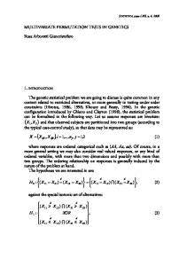
In model (3.1), the two variables of R and P are transformed for diagnostic purpose, and all main effects and two-way interactions between A and S and between A and log P are presented. Now fit the model and the corresponding p-values for testing H0 : βi = 0, i = 1, . . . , 5, are summarized in Table 7. Table 7 indicates that the permutation tests determine that all main effects are significant with level 5%, while usual t-tests conclude that all effects under consideration are not significant. To determine which results are more reliable, we investigate a scatter plot matrix of S , log P and log R only corresponding action equal to one (Figure 1). In the scatter plot matrix, the red solid lines represents the ordinary least square fits and the red dotted lines do LOWESS fits with a smoothing parameter fixed at 2/3. If there are no conditional association of rainfall given action, suitability and prewetness, the scatter plot must show no relations on log R | log P and log R | S . However, we can clearly observe the linear relationship in log R | S , and it can be concluded that the results from usual t-tests are not reliable. After removing the two two-way interactions from model (3.1), refit and define that βˆ T X = βˆ 1 A + ˆβ2 log P + βˆ 3 S . Then, as a summary plot of the regression, we report a scatter plot in Figure 2 of log R versus βˆ T X with imposing LOWESS line with the same parameter configurations as Figure 1. Figure 2 indicates that we can observe a quadratic relation between βˆ T X and log R.

Hye Min Ryu, Min Ah Woo, Kyungjin Lee, Jae Keun Yoo

154

−1.5

−0.5

0.0

3.5

4.0

−2.5

−0.5

0.0

2.0

2.5

3.0

S

1.5

2.0

2.5

−2.5

−1.5

logP

0.0

0.5

1.0

logR

2.0

2.5

3.0

3.5

4.0

0.0

0.5

1.0

1.5

2.0

2.5

Figure 1: A scatter plot matrix of S , log P and log R) only with action equal to one; solid red line, OLS line; blue

-2

-1

0

log R

1

2

3

dotted line, LOWESS line

0

0.5

1

ˆ TX β

1.5

2

2.5

Figure 2: A scatter plot of βˆ T X and log R)

4. Discussions To determine whether each coefficient is equal to zero or not, usual t-tests are popular choice among others in linear regression to usual practitioner, because all statistical packages provide the statistics and their corresponding p-values. Under smaller samples (especially with non-normal errors) the tests often fail to detect the statistical significance correctly. To overcome this deficit, we propose a permutation approach by adopting a sufficient dimension reduction methodology. For this, first we define general predictor hypothesis that contain contrasts. To implement the proposed permutation approach, first, a reference statistics is computed through measuring the distances between the OLS estimates and restricted OLS estimates under user-selected predictor hypothesis. By linearly transformed predictors following the predictor hypothesis and permuting them, we obtain permutation samples. From each permutation sample, the same statistics as the reference one are

Permutation Predictor Tests in Linear Regression

155

computed. Then the percentages that the permuted statistics are bigger than or equal to the reference one are reported as p-values to just the predictor hypothesis. According to numerical studies, the proposed method provides higher powers than usual t-tests regardless of sample sizes and distributions of errors; however, it tends to produce higher observed levels. The proposed permutation tests are not always a winner over usual t-tests; however, it provides additional reliable evidences with smaller samples to determine whether or not each regression coefficient is equal to zero. Therefore, if one uses both tests, it is out of question that they can make more correct decisions. The R codes for the proposed tests are available upon requests.

References Cook, R. D. (1998) Regression Graphics, Wiley, New York. Cook, R. D. and Weisberg, S. (1991). Discussion of sliced inverse regression for dimension reduction by K.C. Li. Journal of the American Statistical Association, 86, 328–332. Cook, R. D. and Weisberg, S. (1999). Applied Regression Including Computing and Graphics, Wiley, New York. Kutner, M. H., Nachtsheim, C. J., Neter, J. and Li, W. (2005). Applied Linear Statistical Models, 5th edition, McGraw-Hill/Irwin, New York. Yin, X. and Cook, R. D. (2002). Dimension reduction for the conditional kth moment in regression. Journal of Royal Statistical Society, Series B, 64, 159–175. Received February 19, 2013; Revised March 18, 2013; Accepted March 25, 2013