A Study of Subsonic Turbulent Jets and Their ... - TFD Chalmers

T HESIS FOR THE D EGREE OF D OCTOR OF P HILOSOPHY IN T HERMO AND F LUID D YNAMICS

A Study of Subsonic Turbulent Jets and Their Radiated Sound Using Large-Eddy Simulation N IKLAS A NDERSSON

Division of Fluid Dynamics Department of Applied Mechanics C HALMERS U NIVERSITY OF T ECHNOLOGY Göteborg, Sweden, 2005

A Study of Subsonic Turbulent Jets and Their Radiated Sound Using Large-Eddy Simulation N IKLAS A NDERSSON ISBN 91-7291-679-6

c N IKLAS A NDERSSON , 2005 Doktorsavhandling vid Chalmers tekniska högskola Ny serie nr 2361 ISSN 0346-718X Division of Fluid Dynamics Department of Applied Mechanics Chalmers University of Technology S E-412 96 Göteborg, Sweden Phone: +46-(0)31-7721400 Fax: +46-(0)31-180976

Printed at Chalmers Reproservice Göteborg, Sweden, 2005

A Study of Subsonic Turbulent Jets and Their Radiated Sound Using Large-Eddy Simulation N IKLAS A NDERSSON Division of Fluid Dynamics Department of Applied Mechanics Chalmers University of Technology

Abstract Stricter noise regulation for near-ground operations has made noise reduction in commercial aircraft a topic of growing interest in the aerospace industry. To meet airworthiness requirements new noise reduction technologies have to be developed and numerical methods for correct assessment of these technologies are desirable. This thesis deals with predictions of near-field flow and far-field acoustic signature of subsonic turbulent single-stream and dual-stream jets at isothermal and heated conditions. The flowfield predictions are obtained using large-eddy simulation (LES), and Kirchhoff ’s surface integration technique is used to extend the acoustic domain to far-field locations. In all cases studied, the nozzle geometry is included in the calculation domain. For the single-stream jet, predicted near-field flow statistics and farfield sound pressure levels (SPL) are both in good agreement with experiments. Predicted SPL for all observer locations, where evaluated, are within a deviation of 3.0 dB from measured levels and for most locations within a deviation of 1.0 dB. For the specific cases studied, Mach 0.75 jets, only small differences in radiated sound could be identified between an isothermal jet and a jet with temperature twice that of the surrounding fluid. The effects of changes in inflow conditions, Reynolds number and subgrid-scale (SGS) model on the flowfield and acoustic signature were investigated. Only minor changes could be identified in the predictions of flow statistics and radiated sound. For the dual-stream jet, changing the subgrid-scale filter width and introducing a TVD limiter gave significant changes in the shear layer flow. Sound radiated in the upstream direction was shown to depend appreciably on the initial shear layer development. Vortex generators placed on the outside wall of the inner nozzle were found to effectively break up ring-shaped vortical structures in the initial inner shear layer region and speed up the mixing between the core and bypass streams. Keywords: CAA, Aeroacoustics, Jet Noise, LES, Kirchhoff, Heated Jets, Coaxial Jets, Two-Point Space-Time Correlations iii

List of Publications This thesis is based on the work contained in the following papers: I N. Andersson, L.-E. Eriksson and L. Davidson, 2005, Investigation of an Isothermal Mach 0.75 Jet and its Radiated Sound Using Large-Eddy Simulation and Kirchhoff Surface Integration, International Journal of Heat and Fluid Flow, 26(3), 393–410 II N. Andersson, L.-E. Eriksson and L. Davidson, 2005, Large-Eddy Simulation of Subsonic Turbulent Jets and Their Radiated Sound, AIAA Journal 43(9) 1899–1912 III N. Andersson, L.-E. Eriksson and L. Davidson, 2005, Effects of Inflow Conditions and Subgrid Model on LES for Turbulent Jets, The 11th AIAA/CEAS Aeroacoustics Conference, AIAA 2005-2925, May 23-25, Monterey, California IV N. Andersson, L.-E. Eriksson and L. Davidson, 2005, LES Prediction of Flow an Acoustic Field of a Coaxial Jet, The 11th AIAA/CEAS Aeroacoustics Conference, AIAA 2005-2884, May 23-25, Monterey, California

Division of Work Between Authors of the Papers The work leading up to this thesis was done in collaboration with other researchers. The respondent is the first author of all papers on which this thesis is based, and the respondent produced all results. Theoretical work and code development presented in the papers were carried out in discussions with supervisors Lars-Erik Eriksson and Lars Davidson. v

Other Relevant Publications N. Andersson, L.-E. Eriksson and L. Davidson, 2003, Large-Eddy Simulation of a Mach 0.75 Jet, The 9th AIAA/CEAS Aeroacoustics Conference, AIAA 2003-3312, May 12-14, Hilton Head, South Carolina N. Andersson, 2003, A Study of Mach 0.75 Jets and Their Radiated Sound Using Large-Eddy Simulation, Licentiate thesis, Division of Thermo and Fluid Dynamics, Chalmers University of Technology, Gothenburg N. Andersson, L.-E. Eriksson and L. Davidson, 2004, A Study of Mach 0.75 Jets and Their Radiated Sound Using Large-Eddy Simulation, The 10th AIAA/CEAS Aeroacoustics Conference, AIAA 2004-3024, May 10-12, Manchester, United Kingdom

vi

Acknowledgments Of all people who have contributed to the accomplishment of the work reported in this thesis, Caroline definitely deserves to be first in line: thank you for all your support and for loving me – I do not know what I would do without you. I would also like to take this opportunity to thank my parents for believing in me and supporting me at all times. I would like to express my gratitude to my supervisors, Professor Lars-Erik Eriksson, for sharing some of his profound knowledge in compressible flows and numerical methods with me, and Professor Lars Davidson, for all good advice and encouragement. I would like to acknowledge Mattias Billson, Johan Larsson and Jonas Ask who together with me, with great support from Lars-Erik Eriksson and Lars Davidson, initiated the computational aeroacoustics research activities at our department. Sharing experiences, setbacks and successes, we have solved problems together that would have been tough to deal with alone. This study would definitely not have reached this stage without the help from you guys. Special thanks to Mattias Billson for all helpful discussions and encouraging talks. Moreover, our joint code development effort is something that I look back upon as the most fun part of my time as a graduate student. I wish to thank Magnus Stridh and Fredrik Wallin with whom I have had many interesting discussions on various subjects, which have given me new insights and ideas that have been valuable in my work. I would also like to thank all participants in the JEAN and CoJeN projects for fruitful discussions at the project meetings. Special thanks to Peter Jordan and co-workers at Laboratoire d’Etude Aero´ dynamiques, Poiters, France, for providing us with experimental data and for showing interest in our work. Many thanks to Stéphane Baralon and Jonas Larsson at Volvo Aero Corporation for giving me thoughtful advice. Financial support from the EU 5th and 6th Framework Projects JEAN, contract number G4RD-CT-2000-000313, and CoJeN, contract number AST3-CT-2003-502790, is gratefully acknowledged. Finally, I would like to thank my friends and colleagues at the Division of Fluid Dynamics for creating a stimulating working atmosphere. vii

To Caroline

Nomenclature Latin symbols speed of sound specific heat at constant pressure specific heat at constant volume Smagorinsky model coefficients

nozzle outlet diameter energy flux component frequency kinetic energy potential core length pressure Prandtl number energy diffusion vector state vector in equations on conservative form state vector in equations on primitive form cell volume averaged state vector gas constant radial coordinate or distance from source to observer Reynolds number based on the jet diameter "! strain rate tensor # cell face area normal vector %$ %$' )(+*-,./( Strouhal number & & 0 temperature $ time 0 ! Lighthill stress tensor 43546 ( axial, radial and tangential velocity component &21 ! 1,. Cartesian components of velocity vector jet-exit velocity 7 volume 698;: flowfield location ? ! Cartesian coordinate vector component xi

far-field observer location Greek symbols filter width ! Kronecker delta 8;: = characteristic speeds dynamic viscosity ' * ( kinematic viscosity & density ! viscous stress tensor ! subgrid-scale stress tensor

retarded time viscous dissipation ! computational space coordinate vector component

Subscripts

$

total condition freestream or ambient conditions jet, nozzle-exit condition turbulent quantity

Superscripts : spatially filtered quantity resolved fluctuation unresolved quantity spatially Favre-filtered quantity subgrid scale Abbreviations CAA Computational Aero Acoustics CFD Computational Fluid Dynamics CFL Courant-Friedrichs-Lewy DNS Direct Numerical Simulation HBR High Bypass Ratio LDV Laser Doppler Velocimetry LEE Linearized Euler Equations LES Large Eddy Simulation MPI Message Passing Interface RANS Reynolds-Averaged Navier-Stokes SGS Subgrid Scale SPL Sound Pressure Level TVD Total Variation Diminishing

xii

Contents Abstract

iii

List of Publications

v

Acknowledgments

vii

1 Introduction 1.1 Motivation . . . . . . . . . . . . . . 1.2 Turbulent Free Jet . . . . . . . . . 1.3 Jet Noise . . . . . . . . . . . . . . . 1.4 Computational Aeroacoustics . . . 1.5 LES and DNS of Turbulent Jets . . 1.6 Measurements Used for Validation

. . . . . .

1 1 3 5 6 8 9

. . . .

11 11 12 13 15

3 Sound Propagation 3.1 Lighthill’s Acoustic Analogy . . . . . . . . . . . . . . . . . 3.2 Kirchhoff Surface Integration . . . . . . . . . . . . . . . .

17 17 19

4 Numerical Method 4.1 Spatial Discretization . . . . . . . . . . . . . . . 4.1.1 Convective Fluxes . . . . . . . . . . . . . 4.1.2 Diffusive Fluxes . . . . . . . . . . . . . . 4.2 Time Stepping . . . . . . . . . . . . . . . . . . . 4.3 Boundary Conditions . . . . . . . . . . . . . . . 4.3.1 Method of Characteristics . . . . . . . . 4.3.2 Special Treatment of Outlet Boundaries 4.3.3 Entrainment Boundaries . . . . . . . . .

23 24 24 30 31 32 32 34 35

2 Large-Eddy Simulation 2.1 Governing Equations . 2.2 Spatial Filtering . . . . 2.2.1 Favre Filtering . 2.3 Subgrid-Scale Model .

. . . .

. . . .

. . . .

xiii

. . . .

. . . .

. . . .

. . . .

. . . . . . . . . .

. . . . . . . . . .

. . . . . . . . . .

. . . . . . . . . .

. . . . . . . . . .

. . . . . . . . . .

. . . . . . . . . .

. . . . . . . . . .

. . . . . . . .

. . . . . . . . . .

. . . . . . . .

. . . . . . . . . .

. . . . . . . .

. . . . . . . . . .

. . . . . . . .

. . . . . . . . . .

. . . . . . . .

. . . . . . . .

4.4 Evaluation at Retarded Time . . . . . . . . . . . . . . . . 5 Summary of Papers 5.1 Paper I . . . . . . . . . . . . . . . . 5.1.1 Motivation and Background 5.1.2 Work and Results . . . . . . 5.1.3 Comments . . . . . . . . . . 5.2 Paper II . . . . . . . . . . . . . . . . 5.2.1 Motivation and Background 5.2.2 Work and Results . . . . . . 5.2.3 Comments . . . . . . . . . . 5.3 Paper III . . . . . . . . . . . . . . . 5.3.1 Motivation and Background 5.3.2 Work and Results . . . . . . 5.3.3 Comments . . . . . . . . . . 5.4 Paper IV . . . . . . . . . . . . . . . 5.4.1 Motivation and Background 5.4.2 Work and Results . . . . . . 5.4.3 Comments . . . . . . . . . .

. . . . . . . . . . . . . . . .

. . . . . . . . . . . . . . . .

. . . . . . . . . . . . . . . .

. . . . . . . . . . . . . . . .

. . . . . . . . . . . . . . . .

. . . . . . . . . . . . . . . .

. . . . . . . . . . . . . . . .

. . . . . . . . . . . . . . . .

. . . . . . . . . . . . . . . .

. . . . . . . . . . . . . . . .

. . . . . . . . . . . . . . . .

. . . . . . . . . . . . . . . .

. . . . . . . . . . . . . . . .

36 39 39 39 39 40 41 41 41 42 42 42 43 45 45 45 46 48

6 Further Investigation of the CoJeN Coaxial Nozzle/Jet Configuration 51 6.1 Vortex Generator Implementation . . . . . . . . . . . . . 53 7 Concluding Remarks 7.1 Single-Stream Jet . . . . . . . . . . . . . . . . . . . . . . . 7.2 Coaxial Jet . . . . . . . . . . . . . . . . . . . . . . . . . . . 7.3 Recommendations for Future Work . . . . . . . . . . . . .

57 57 59 59

Bibliography

61

A Characteristic Variables

69

B Physical and Computational Space

71

C MPI Implementation

75

Paper I Paper II Paper III Paper IV xiv

Chapter 1 Introduction 1.1

T

Motivation

number of commercial aircraft in service is continuously growing, and airports around the world are growing in size, which increases exposure to air traffic noise in populated areas. Threshold values for noise certification of new aircraft are based on global restrictions on noise generated by air traffic. Moreover, local restrictions for airports with heavy traffic limit operating hours or even impose direct noise penalty costs. Stricter regulations on noise levels in the surroundings of airports have made the abatement of near-ground operation noise an important issue for aircraft and engine manufacturers, and noise generation has now become an important design factor that is taken into consideration early in the construction process. Despite progress in the development of computational fluid dynamics (CFD) solvers, most of the noise prediction methods currently in use in industry are correlations based on empirical databases. The reason for this is the extreme demands for numerical accuracy in computational aeroacoustic (CAA) methods that place high demands on computational resources. However, to be able to account for changes in the flow by new noise reduction techniques or to predict differences in radiated sound in different engine concepts at an early design stage, more explicit approaches are required. With continuously increasing computer capacity and with the possibility to carry out parallel computations on PC clusters, computational aeroacoustics has now, to some extent, become feasible for industrial use. Flow-induced aircraft noise can be divided into two categories: airframe noise and noise generated by the jet engine. The first category includes noise generated by landing gear, high-lift devices and the aircraft fuselage itself and the second includes turbo-machinery noise, HE

1

Niklas Andersson, A Study of Subsonic Turbulent Jets and Their Radiated Sound Using Large-Eddy Simulation core noise and jet noise. At take-off, the main sources of noise are the propelling jet and the engine fan, of which the jet exhaust is usually the strongest noise source at full power. In commercial aircraft, increasing the bypass ratio, i.e. the ratio of mass passing the engine in the bypass duct to the mass passing through the engine core, has given a significant reduction in aircraft noise since the 1960s. However, although an increase of the bypass ratio leads to lower noise levels, the major motivation for this development has not been noise reduction. Rather, the development towards more efficient engines has led to the use of a higher bypass ratio with noise reduction as a positive side effect. The lower noise levels of high-bypass ratio (HBR) engines are directly attributable to the reduction in jet noise resulting from lower jet velocities. Unfortunately, without a step change in technology, the maximum bypass ratio is limited by a number of factors, e.g. the length of the fan blades, engine weight, rotor speed and engine nacelle drag, and large engines are currently very close to this limit. Consequently, the possibility for reducing jet noise by increasing the bypass ratio is rapidly decreasing. Other techniques to lower noise levels have been investigated in the past decades. Among these concepts, many are of a mixing enhancement nature, e.g. chevrons, lobed mixers and tabs. The lobed mixer efficiently evens out differences in the velocity of the core flow and the bypass flow, which reduces the exhaust velocity and hence the sound generated. Chevrons and tabs are both devices added to the nozzle geometry that protrude into the flow and generate axial vorticity and thereby enhance the mixing of core, fan and ambient air streams. While these noise-reducing concepts have proved to be able to lower noise levels (e.g. Saiyed et al., 2000; Nesbitt et al., 2002), the reduction comes with a penalty on efficiency. The contradiction of noise reduction for near-ground operation and requirements for higher thrust and engine efficiency at cruise conditions will probably be common in all new noise-reducing concepts. Furthermore, requirements for higher thrust are often satisfied by increasing the flow through existing engines with only minor modifications, which leads to higher exhaust velocities and temperatures and increases the contribution of the jet to the overall noise. Part of the work presented in this thesis has been conducted within the EU 5th framework programme JEAN1 , which was an European project investigating the physics behind noise generation in isothermal and heated single-stream jets. In this project, jet noise mechanisms 1

JEAN – Jet Exhaust Aerodynamics & Noise, Contract number: G4RD-CT-2000000313

2

CHAPTER 1. INTRODUCTION were investigated both numerically and experimentally and various known methodologies for noise prediction were tested and compared for a few test cases. In the continuation of that project, CoJeN2 , the flowfield and radiated sound of a high-subsonic coaxial nozzle/jet configuration is being investigated. The work reported in Paper IV was done within the framework of the latter of the two projects. The objective of CoJeN is to develop and validate prediction tools that can be used by the aerospace industry to assess and optimize jet noise prediction techniques. The aim is to provide design tools that can be used to develop low-noise nozzles for HBR engines. For prediction techniques to be useful to industry, the methods must cope with realistic jet flows such as coaxial jet configurations with high velocities, significant velocity and temperature gradients, and arbitrary nozzle geometries. Hence, the ability to capture the initial flow physics becomes very important. LES is not currently feasible for industrial design use because of long turnover times and a restriction to fairly simple geometries. However, new noise-reducing concepts will arise from a better understanding of the source mechanisms. To evaluate the performance of these new concepts, reliable methods for modeling the source mechanisms must be available. The results of a detailed LES can be used to gain a more realistic picture of the flow physics and thus be useful in the development of tools for industrial use. For example, higher-order statistics important for the understanding of noise generation, such as two-point space-time correlations, can be evaluated. Detailed information on the statistical character of the flow can later be used to develop prediction techniques based on noise generation mechanisms. This is the main objective of the present work.

1.2

Turbulent Free Jet

The turbulent free jet is an example of a free shear flow, i.e. a flow with mean flow gradients that develop in the absence of boundaries (George, 2000). This kind of flow is characterized by a main flow direction in which the velocity is significantly greater than in the transverse direction. The gradients in the transversal direction are also much larger than those in the main direction. These kinds of flows are common both in nature and in engineering applications. Examples are the residual gases spread into the atmosphere by a furnace chimney and the propelling jet of an aircraft engine. The turbulent jet is separated from its non-turbulent surroundings by an interface often referred to 2

CoJeN – Computation of Coaxial Jet Noise, contract number: AST3-CT-2003502790.

3

Niklas Andersson, A Study of Subsonic Turbulent Jets and Their Radiated Sound Using Large-Eddy Simulation as the viscous super layer, by analogy with the viscous sublayer of a boundary layer, or the Corrsin super layer after its discoverer (Hinze, 1975; George, 2000). The shape of the interface is random and continuously changing and its thickness is characterized by the Kolmogorov microscale (George, 2000). The flow in these outer regions of the jet is therefore intermittent in nature, i.e. sometimes turbulent and sometimes not, as the shape of the jet and its interface with the surroundings changes. The level of intermittancy increases radially outwards through the jet shear layer. Minimum intermittancy is found in the radial location in which the shear is highest (Wygnanski & Fiedler, 1969). The shape of the interface is strongly affected by the turbulent flow in the jet, and then mainly by the larger structures of the flow (Hinze, 1975; George, 2000). The motion of the interface induces irrotational fluid motion of the surrounding fluid. The amount of turbulent fluid continuously increases downstream due to entrainment, i.e. fluid is entrained to the turbulent jet from its surroundings. The entrainment process causes the jet to spread in the transversal direction, and the jet flow can therefore never reach homogeneity (George, 2000). As long as the jet remains turbulent, the range of scales present in it will increase as a result of its increasing size. In the entrainment process, mass is continuously added to the turbulent jet, but no momentum is added. Figure (1.1) shows the development of a single-stream jet. Highvelocity fluid is continuously added through a nozzle into stagnant surroundings. As it exits the nozzle, the flow of the high-velocity fluid is fully aligned with the nozzle wall, and a core region of potential flow is formed. A shear layer is generated between the high-velocity fluid and its surroundings. The thickness of this shear layer depends on the thickness of the boundary layer at the nozzle exit. Due to entrainment of ambient fluid, the shear layer grows in size downstream. As the width of the shear layer increases, the radial extent of the potential core region decreases and more and more of the flow becomes turbulent. Shortly after the potential core closure, the entire jet is turbulent and thus fully developed. The jet becomes self-preserving or self-similar in the fully developed region. This means that profiles of mean flow quantities can be collapsed by proper scaling. It has long been assumed that these selfsimilar profiles are independent of initial conditions for all quantities and therefore universal for all jets. This assumption has been questioned by George (1989), however. 4

CHAPTER 1. INTRODUCTION core region

transition fully developed region

region

Figure 1.1: Flow regions in a developing jet

1.3

Jet Noise

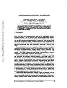
Investigation of jet noise was more or less initiated in 1952 when Lighthill proposed his acoustic analogy in the first of his two-part paper on aerodynamically generated sound (Lighthill, 1952, 1953). These publications focused mainly on the sound generated by turbulent jets, but the acoustic analogy presented therein has been used extensively for numerous applications in the area of aeroacoustics. In addition to the work of Lighthill, a number of researchers such as Curle (1955); Lilly (1958); Ffowcs Williams (1963); Ffowcs Williams & Hawkings (1969); Ribner (1969) have made significant contributions to the theory and applications of acoustic analogies. A thorough review of the development of acoustic analogies can be found in Crighton (1975). The understanding of flow-induced noise, for example jet noise, is strongly coupled to the understanding of turbulence since the sources of sound are defined by the turbulent flow itself. Fifty years ago, when jet noise research was initiated, turbulence was regarded as consisting of randomly distributed small eddies. Thus the research focused on the noise generated by fine-scale structures. The focus changed with the discovery of large turbulence structures in free shear flows in the early 1970s and it was believed that, for high-speed jets, the dominant part of the sound generated was generated by these large structures. More recent analysis has shown that both the fine scales and the larger structures are responsible for the noise that is generated (Tam, 1998). In jet flows, the sound-generating structures are convected downstream by the mean flow. It can be shown that moving sources tend to radiate more sound in the direction in which the source is transported (Tam, 1998; Ribner, 1969). Moreover, the sound generated is affected by the mean convection such that when the wave front propagates through the jet on the way to the far-field region its path tends to bend away from the jet axis. The reason for this is that the con5

Niklas Andersson, A Study of Subsonic Turbulent Jets and Their Radiated Sound Using Large-Eddy Simulation vection velocity is highest in the centerline regions (A) and lower in the outer jet regions (B), see Figure (1.2). This effect is referred to as refraction and creates a cone of relative silence downstream of the noise-generating region since less sound is radiated in this direction. The refraction effect is more noticeable for jets with a higher temperature than the surrounding fluid since the speed of sound then varies over the jet cross section (Tam, 1998).

Nozzle

Turbulent mixing layer

Figure 1.2: Refraction of a sound wave generated at position in the shear layer and propagating through the jet. A wave front defined by line is propagating downstream at a velocity defined by the speed of sound and the local flow velocity. The flow velocity is higher in than in , which results in a tilting of the wave front towards line .

According to Ribner (1969), the sound generated by a turbulent jet can be separated into two parts. These are the sound generated by interaction of turbulence fluctuations and the sheared mean flow and the sound generated by turbulence fluctuations interacting with themselves; for greater detail see e.g. Ribner (1969). The two sound components are often referred to as shear noise and self noise, respectively. The self noise is radiated equally in all directions whereas the shear noise gives a dipole-like contribution. Superimposed, these two contributions give an ellipsoid-shaped sound radiation pattern, with the most sound radiated along the jet axis. Adding the effect of convection, the part of the sound that is radiated downstream of the jet is significantly larger than the part radiated in the upstream direction. Refraction significantly decreases the sound radiated along the jet axis. The contribution to the overall sound of the two components and the effect of convection and refraction on the pattern of radiated sound are depicted in Figure (1.3). 6

CHAPTER 1. INTRODUCTION

=

+ self noise

shear noise

refraction

convection

Figure 1.3: Superimposition of the noise generated by the turbulence itself, self noise, and the noise generated by interaction of the mean shear flow and turbulence, shear noise, gives the upper right sound pattern. Convection and refraction affect the pattern of radiated sound, and the result is the directional sound pattern in the lower right figure.

1.4

Computational Aeroacoustics

Using a grid fine enough in the far-field regions to minimize the introduction of sound propagation errors, the acoustic field can be obtained directly from the flowfield simulation. This requires a detailed numerical compressible flow simulation, e.g. direct numerical simulation (DNS), see for example Freund (2001) and Mitchell et al. (1999), or LES, as in e.g. Bogey et al. (2000a, 2003); Bogey & Bailly (2003, 2004, 2005b) and Mankbadi et al. (2000). In DNS, all scales of the turbulent flowfield are computed accurately, which requires a mesh fine enough to capture even the smallest scales of the flow, whereas in LES only the large scales of the flow are resolved and the influence on these large scales of the smaller, unresolved scales is modeled using a subgrid-scale model. With the computational resources available today, DNS is restricted to fairly simple geometries and low Reynolds number flows. Moreover, it is believed, see Mankbadi (1999), that large scales are more efficient than small ones in generating sound, which justifies the use of LES for sound predictions. To save computational time, a hybrid approach can be used in which the computational problem is divided into two parts. An LES can be used to obtain the unsteady non-linear near field, which in the jet noise case corresponds 7

Niklas Andersson, A Study of Subsonic Turbulent Jets and Their Radiated Sound Using Large-Eddy Simulation to the hydrodynamic jet region. The acoustic field is then extended to far-field observer locations using, for example, the surface integration formulation by Kirchhoff (1883) as in e.g. Lyrintzis (1994) and Freund et al. (1996). Using a hybrid approach may even lead to noise predictions of higher quality than a direct approach since the amount of numerical dissipation to which the sound waves are exposed is decreased. Furthermore, the frequency cut-off is often higher in the integration surface regions than in the far field (Uzun, 2003; Uzun et al., 2005). Another approach is to use a less computationally expensive Reynolds-Averaged Navier-Stokes (RANS) calculation to obtain a timeaveraged flowfield. Information about length and time scales in the time-averaged flowfield can then be used to synthesize turbulence in the noise source regions. The acoustic field is obtained by solving a set of equations, e.g. the linearized Euler equations, with source terms obtained from the synthesized flowfield, see Billson (2004). This method is promising since it is possible to make simulations of high Reynolds number flows with reasonable computational efforts. Information on the acoustic far field can also be obtained by using RANS data as input for a statistical method based on an acoustic analogy as in e.g. Hunter & Thomas (2003), Farassat et al. (2004) and Self & Bassetti (2003) or by the use of RANS data in combination with semi-empirical relations as done by e.g. Tam & Auriault (1999), Tam & Pastouchenko (2002) and Tam & Ganesan (2004).

1.5

LES and DNS of Turbulent Jets

LES and DNS have been used for jet flow applications in a number of investigations. These primarily study jets at moderate Reynolds number due to the high computational costs of making simulations of a high Reynolds number jet. Many of these studies have been carried out to predict jet noise. However, as jet flows are free shear flows frequently occurring in both nature and industrial applications, it is interesting to study the jet in itself. Some studies are thus pure investigations of flow phenomena. The feasibility of using LES for both the flowfield and the radiated sound from a high-subsonic 6.5 10 Reynolds number jet has been discussed by Bogey et al. (2000a, 2003, 2001). In the work presented in Bogey et al. (2000a, 2003), the acoustic field was obtained directly from the flow simulation. Noise-generation mechanisms were found to be relatively independent of the Reynolds number. In the work by Bogey et al. (2001) the acoustic analogy of Lighthill (1952) was used in combination with compressible LES to obtain the acoustic field. Bo

8

CHAPTER 1. INTRODUCTION gey & Bailly (2003, 2005a) investigated the effects of inflow condi= and the radiated sound of a high Reynolds numtions on the flowfield ' ber, 4.0 10 , Mach 0.9 jet. Both the flow development and the emitted sound were shown to depend appreciably on inlet parameters. Bogey & Bailly (2004) investigated the effects of Mach and Reynolds number on subsonic jet noise. Bodony & Lele (2004) investigated the changes in the jet mean field and far-field sound when simulating jets with different temperatures and Mach numbers. Results were found to be in agreement with published data (Tanna, 1977). Freund (2001) used DNS to investigate sources of sound in a Mach 0.9 jet at a Reynolds ' number of 3.6 10 . In this work the part of the Lighthill source that may radiate to the far field was isolated using Fourier methods. It was found that the peak of the radiating source coincides neither with the peak of the total source nor the peak of turbulence kinetic energy. Shur et al. (2003) made simulations of a cold Mach 0.9 jet at a Reynolds number of 1.0 10 . Radiated sound was successfully pre= dicted using the surface integral formulation by Ffowcs Williams & Hawkings (1969). The simulation was made using only 5.0 10 cells. This work was done with the monotone-integrated LES (MILES) approach, where the subgrid-scale model is essentially replaced by the numerical dissipation of the numerical method. Zhao et al. (2001) made an LES of a Mach 0.9 jet at Reynolds number 3.6 10 and a jet at Mach 0.4 and a Reynolds number of 5.0 10 . In that study, radiated sound was obtained both directly from the LES and by using Kirchhoff surface integration. The effect on the radiated sound of the subgridscale model was investigated. It was found that using a mixed subgridscale model resulted in both higher turbulence levels and sound levels. = Uzun (2003); Uzun et al. (2005) made LES of a high-subsonic (Mach 0.9) single-stream jet at a Reynolds number of 4.0 10 . Sound pressure levels obtained using surface integral methods, e.g. Kirchhoff and Ffowcs William & Hawkings, were compared to results obtained using a volume integral method (Lighthill’s acoustic analogy). The results obtained using the surface approaches were found to be comparable with the results obtained using Lighthill integration.

1.6

Measurements Used for Validation

Measurements for the single-stream jet configuration were made by Jordan et al. at the MARTEL facility of CEAT (Centre d’Etudes Aero´ dynamiques et Thermiques), Poiters. Two-component single-point and mono-component two-point measurements were made using Laser Doppler Velocimetry (LDV). The acoustic field was sampled using an arc of 9

Niklas Andersson, A Study of Subsonic Turbulent Jets and Their Radiated Sound Using Large-Eddy Simulation microphones at 30 jet diameters and 50 jet diameters from the jet exit, respectively. These measurements were made within the framework of the JEAN project. For greater detail on the experimental set-up see Jordan et al. (2002a,b); Jordan & Gervais (2003). These measurements have also been reported in part by Power et al. (2004). No experimental data for validation of the LES predictions for the coaxial jet configuration are available at this stage of the CoJeN project. At a later stage, single-point multi-component statistics and spatial correlations will be available for validation of the predicted flow data, and the predicted acoustic signature will be evaluated using far-field acoustic measurements.

10

Chapter 2 Large-Eddy Simulation has recently been established as a nuL merical approach for the simulation of turbulent flows in situations in which detailed information on turbulence characteristics and flow ARGE EDDY SIMULATION

physics is desirable and DNS is far too expensive. LES enables accurate representation of large scales of the flow, i.e. as accurate as possible considering the errors introduced by the numerical method and the assumptions made. The effects on the large, resolved scales of those not resolved are modeled using a subgrid-scale model. By refining the mesh, LES approaches DNS, where all scales of the flow should be represented accurately. However, only resolving the larger scales significantly decreases the computational effort needed, making LES more feasible for non-academic flows. Furthermore, the larger eddies are directly affected by the boundary conditions, carry most of the Reynolds stresses and must be computed, whereas the small-scale turbulence is weaker, contributing less to the Reynolds stresses. Thus, it is less critical to represent these smaller scales accurately. The smaller scales are also more nearly isentropic and have nearly universal characteristics and are therefore more amenable to modeling (Wilcox, 1998).

2.1

Governing Equations

The compressible form of the continuity, momentum and energy equations in which the viscous stress and heat flux have been defined using Newton’s viscosity law and Fourier’s heat law, respectively, are often referred to as the Navier-Stokes equations:

$

& 1 ? ! 11

!( '

(2.1)

Niklas Andersson, A Study of Subsonic Turbulent Jets and Their Radiated Sound Using Large-Eddy Simulation

!(

( & $

!

& 1 $

/ ( & 1 ' : ?

! / ( & 1 1 ' : ?

1 ?

?

? !

0

! ?

?

(2.2)

? &1

! ! (

(2.3)

in Eqns. (2.2) and (2.3) is the viscous stress defined by

where

"!

! '

"! :

is the strain-rate tensor given by

"! '

1

?

!

!

1

? !

(2.4)

(2.5)

in Eqn. (2.3) denotes the Prandtl number. In the present work the system of governing equations, Eqns. (2.1– 2.3), is closed by making assumptions on the thermodynamics of the gas considered. It is assumed that the gas is a thermally perfect gas, i.e. it obeys the gas law ' - 90 (2.6)

where is the gas constant. Furthermore, the gas is assumed to be calorically perfect, which implies that internal energy and enthalpy are linear functions of temperature.

'

0 0 :

'

'

(2.7)

Here, is the specific heat at constant pressure. Moreover, the viscosity, , is assumed to be constant.

2.2

Spatial Filtering

By low-pass filtering the governing equations in space, flow features that are smaller than an externally specified characteristic filter width are effectively removed from the solution. The basic idea is that structures larger than the filter width should be left unaffected by the filter operation and that the effect of scales smaller than the filter width are removed and must be modeled. In the present work the low-pass filtering procedure is considered to be coupled to the discretization in the finite-volume method solver, which means that it corresponds to a box filter and that the characteristic length scale is related to the local grid cell size. 12

CHAPTER 2. LARGE-EDDY SIMULATION

2.2.1 Favre Filtering A spatial Favre filter is used in this work, i.e. a mass weighted spatial filter. Favre filtering is a common filtering approach for compressible flows since it results in governing equations in a convenient form, i.e. a form very similar to that of the unfiltered equations. Moreover, using a filter approach in which fluctuations in density are considered would lead to more complicated subgrid-scale terms. For example, with such a filter, subgrid-scale terms would appear in the continuity equation, terms that would need modeling of their own (Guerts, 2004). Using Favre filtering, the flow properties are decomposed as follows

'

(2.8)

where is a Favre-filtered, resolved quantity and is the unresolved part of . The Favre-filtered part of is obtained as follows

'

(2.9)

in contrast to Favre time averaging

' '

and hence

(2.10) (2.11)

The Favre-filtered continuity, momentum and energy equations are obtained by applying the filtering operation, Eqn. (2.9), directly to the governing equations, Eqns. (2.1–2.3), which implies !( & 1 ' $ (2.12) ? !

( & $

& 1 $

!(

/ ( & 1 ' : ?

: !

! / ( ! ! & 1 1 ' : ? ? ! ? ? 0 1 ? ? ?

! ! : ! ! 1 1 1 ? 1 1 1

(2.13)

? &1

! ! )(

(2.14)

!

where and are the Favre-filtered viscous stress tensor and subgridscale viscous stress tensor, respectively. These are here defined as 13


! '

and

! ' :

"!

In Eqn. (2.15),

"! :

! : ! 1 1 1 1

!

(2.15)

1 ! 1 1 ! 1 1 ! 1

! : ! /( &1 1 1 1

' :

(2.16)

is the Favre-filtered rate of strain tensor given by

"! '

?

! 1 !

1

?

(2.17)

As can be seen in Eqn. (2.16), the subgrid-scale stress tensor is a tensor built up of products of resolved and unresolved quantities. These terms appear when the spatial filter is applied to the convective term in the momentum equation. Terms I–III in Eqn. (2.16) are often referred to as Leonard stress, cross term and subgrid-scale Reynolds stress, respectively. When the convective terms in the energy equation are filtered, a term analogous to the subgrid-scale stress term appears. This term, in Eqn. (2.14), is later referred to as a subgrid-scale denoted by heat flux term and is given by

' :

$( :

(3.7)

which, assuming that the acoustic compression-expansion processes in the flow are adiabatic, is related to a corresponding pressure fluctuation as & > $ ( ' & > $ ( (3.8) Using Eqn. (3.5) together with Eqn. (3.8), the sound pressure level in a far-field observer location can be estimated by integration over a volume containing all sound-generating sources. It is important to note that no interaction between the propagating sound wave and the flowfield in which it is propagating is explicitly considered when the integral form of the analogy is used, which for example means that no refraction or convection effects are taken into account. The equation produced by this pioneer work has later been modified in several ways to include, for example, the effects of the mean-flow acoustic interactions, flow inhomogeneities and solid surfaces. Among other, researchers such as Curle (1955); Lilly (1958); Ffowcs Williams (1963); Ffowcs Williams & Hawkings (1969); Ribner (1969) have made significant contributions to the theory proposed by Lighthill so as to make the use of the acoustic analogy applicable to a wider range of problems. Each of these theories differs in the definition of the noise source and the source definitions are all different from Lighthill’s quadrupole source. Due to this non-uniqueness in noise source definition, it has recently been questioned by Tam (2001, 2002) whether the Lighthill quadrupole source term is a real noise sources or not. A thorough review of the development of the acoustic analogy is given in Crighton (1975). 19


3.2

Kirchhoff Surface Integration

Kirchhoff integration is a method for predicting the value of a property governed by the wave equation at a point outside a surface enclosing all generating structures (Lyrintzis, 1994). The method was originally used in the theory of diffraction of light and in other problems of an electromagnetic nature (Kirchhoff, 1883) but has recently been extensively used for aeroacoustic applications. The integral relation is given by

&

$( '

:

$

&>

(

(3.9)

denotes that the expression within brackets is to be evaluated at a retarded time, i.e. emission time. is again the speed of sound in the far-field region. The variable that is to be evaluated in this case is the surface pressure. denotes the surface enclosing all sound-generating structures and denotes the direction normal to the surface. Surface must be placed in a region where the flow is completely governed by a homogeneous linear wave equation with constant coefficients (Freund et al., 1996). The strength of the sources in the hydrodynamic jet region decays slowly downstream, which means that the downstream end of a closed surface will be located in regions of considerable hydrodynamic fluctuations. It is thus common practice to use Kirchhoff surfaces that are not closed in the upstream and downstream ends, see Figure (3.2). Freund et al. (1996) showed that the errors introduced by using such surfaces are small if the main portion of the sound sources are within the axial extent of the surface and if lines connecting observer locations with locations in the hydrodynamic region, representing the main sources of sound, intersect the surface. Rahier et al. (2003) found that the downstream closing surface makes only a minor contribution to the radiated sound. Greater detail on the Kirchhoff surface integration method is given in e.g. Freund et al. (1996) and Lyrintzis (1994). All simulations described in this thesis have been done using jetfitted Kirchhoff surfaces open in the downstream end. For each simulation the integration surface is defined by a set of grid nodes and expands in the radial direction as the mesh stretching increases. This prevents the surface from entering the hydrodynamic jet region when the jet grows in size downstream of the nozzle exit. The Kirchhoff surface integral method is less computationally expensive and storage demanding than a method based on volume integrals, e.g. Lighthill’s acoustic analogy, since it is only surface data that

20

CHAPTER 3. SOUND PROPAGATION

Kirchhoff surface

> Nozzle

Kirchhoff surface Figure 3.2: Sound generated in the shear-layer location, , is propagated in the Navier-Stokes solver and extracted from the Kirchhoff surface to the far-field observer, . The surface is open in the downstream end to prevent it from entering the hydrodynamic jet region.

must be stored and evaluated. Moreover, the integrand includes only first-order derivatives, while the integrand in Lighthill’s acoustic analogy contains second-order derivatives in time or space depending on the formulation used. One of the main strengths of the Kirchhoff surface integral approach, contrary to many other methods, is that, as long as all sources of sound, flow inhomogeneities and objects that in some way affect the radiated sound are bounded by the surface, all these effects are taken into account. This means, for example, that no extra treatment is needed to be able to predict the effects of refraction and convection. This is one of the attractive features of this method. Moreover, both a strength and a weakness of the surface integral approach is the effect of numerical dissipation on the predicted sound. Acoustic waves approaching the integration surface will be low-pass filtered by the numerical method. A result of this artificial dissipation is that spurious high-frequency noise not supported by the mesh and scheme will be filtered out and thus not contribute to the predicted far-field sound. On the other hand, the numerical dissipation affects the ability to capture the high-frequency range of the acoustic pressure spectra, and thus the quality of the prediction depends strongly on the mesh resolution in the Kirchhoff surface region. The ideal situation would be to place the integration surface as far as possible from the sources to ensure that all non-linearities are enclosed by the integration sur21

Niklas Andersson, A Study of Subsonic Turbulent Jets and Their Radiated Sound Using Large-Eddy Simulation face. However, the distance from the source to the surface is limited by the numerical dissipation introduced by the method. Using the surface integral method proposed by Ffowcs Williams & Hawkings (1969) on a porous surface formulation allows the surface to enter regions with weak hydrodynamic fluctuations, which means that the surface can be placed somewhat closer to the sources of sound than when the Kirchhoff formulation is used, see e.g. Shur et al. (2003), Rahier et al. (2003), Uzun (2003) and Uzun et al. (2005). If placed in the linear acoustic field, however, the Kirchhoff surface formulation and the formulation by Ffowcs William & Hawkings are identical. Moreover, Uzun (2003) and Uzun et al. (2005) found the results obtained using the two surface integration methods to be similar for integration surfaces placed rather close to the jet.

22

Chapter 4 Numerical Method

T

code used for the large-eddy simulations is one of the codes in the G3D family of finite-volume method, block-structured codes developed by Eriksson (1995). These codes solve compressible flow equations on conservative form on a general structured boundary-fitted, curve-linear non-orthogonal multi-block mesh. To enhance calculation performance and enable simulations with a large number of degrees of freedom, routines for parallel computations based on the MPI1 libraries have been introduced in the code. Appendix C describes the MPI implementation in more detail. This chapter gives an overview of the numerical scheme and boundary conditions used. Detailed descriptions of these subjects are given in Eriksson (1995) and Eriksson (2005). For convenience, the Favre-filtered Navier-Stokes equations, Eqns. (2.12–2.14), are written in a more compact form: ' $ ? (4.1) HE

where

'

!

1

(4.2)

and

' 1

1

1 : ! : ! ! ! 1 1 1 : : 1 ! & !

Message Passing Interface

23

! )(

(4.3)


! ! The stress tensors, and , in Eqn. (4.3) are defined by Eqn. (2.15) and Eqn. (2.23), respectively. Eqn. (4.1) is discretized on a structured non-orthogonal boundary-fitted mesh. Integrating Eqn. (4.1) over an arbitrary volume gives 7 7 ' ? (4.4) $ Using the Gauss theorem to rewrite the second volume integral to a surface integral and introducing as the cell average of over implies 7 # ' $ (4.5)

# '

#

In Eqn. (4.5), is the face area normal vector, i.e. an area with a direction. The integral of the fluxes is approximated using the area of cell faces and the face average flux

! ! # ' # !" 8

(4.6)

Eqn. (4.4) can now be rewritten as

! ! 7 # ' $ !" 8

(4.7)

The total flux, , is divided into a convective part and a diffusive part in the following way: 1 : ! : ! ! ! ' : ! ! ! )( (4.8) 1 1 :

1

1

1

&

where the first part is the convective, inviscid part and the second the diffusive, viscous part.

4.1

Spatial Discretization

4.1.1 Convective Fluxes The convective flux across a given cell face is calculated with a userdefined upwind scheme based on the propagation direction of the characteristic variables at the cell face. This work has used a low-dissipation 24

CHAPTER 4. NUMERICAL METHOD third-order upwind scheme. The analysis of characteristic variables is made using the solution variables on primitive form , which can be estimated from the variables on conservative form with second-order accuracy.

'

1

!

(4.9)

Linearizing the governing equations on primitive form around a point located on the cell face and considering only plane waves parallel to the cell face gives a one-dimensional system of hyperbolic equations. This equation system can be decoupled by transformation to characteristic variables, see Appendix A. Estimates of the characteristic speeds are computed using face values of the state vector obtained as averages of the values in two adjacent cells according to

'

&

(

(4.10)

Superscript in Eqn. (4.10) denotes average, and subscripts 2 and 3 denote the cells on each side of the face, see Figure (4.1).

Face A

Figure 4.1: Cells used to obtain estimates of the inviscid fluxes across cell face A

Using the cell face values in Eqn. (4.10), the characteristic speeds are obtained as

8 '

'

'

= '

'

# ! 1 ! 8 8 8 8:

# !# ! # !# !

(4.11)

The characteristic variables on the face are obtained using upwinded face values of the primitive variables. Two versions of on the cell 25

Niklas Andersson, A Study of Subsonic Turbulent Jets and Their Radiated Sound Using Large-Eddy Simulation face are calculated, one obtained by upwinding from the left and one obtained by upwinding from the right according to

' 8 8 ' 8

8

(4.12)

8

where superscripts and denote left and right, respectively. , , and are constants defining the upwinding scheme for a four-point stencil.

The sign of the characteristic speeds gives the direction in which local waves in the vicinity of the cell face are traveling in relation to the cell face normal vector. Each of the five characteristic variables are calculated using state vector values upwinded in the direction of the corresponding characteristic speed, i.e. either the left upwinded version or the right upwinded version of is used. The characteristic variables are obtained as follows

698 ' 6

#8 '

'

'

6= '

1

#8 #8

6 6

: &

# !# !

: #

(

1 8 # #

#8 #8

# # 1

# ! ! 1 # # ( & : # ! ! 1 # # ( &

: #

#8 1 8

#8 #8

#

# 1 #

(4.13)

where again superscripts and denote left and right, respectively. The characteristic variables are transformed back to solution variables on primitive form using the following relations 26

CHAPTER 4. NUMERICAL METHOD

'

698

8 ' 1 1

' '

1

'

# #

&

:

6

#8 #8 6= (

6

:

#8 #8 # # # 6 #8 #8 # #

#8 # # #8 # #

: 6 # 6 6=

# #

# 6 #8 #8 # # # 6 #8 #8 # #

#

&

6

:

:

&

&

6

6 = (

6

6 = (

6 = ( (4.14)

The convective flux over the cell face can be estimated by inserting the face values obtained in Eqn. (4.14) into the inviscid part of Eqn. (4.8). The convective scheme used in all the simulations reported in this thesis is a combination of centered and upwind biased components that ˚ have been used with good results for free shear flows by Martensson et al. (1991) and, more recently, for shock/shear-layer interaction by Wollblad et al. (2004) and Wollblad (2004). The coefficients of the lowdissipation upwind scheme used for estimating the convective flux over ( a cell face are derived using a third-order polynomial & ? to represent the variation of the flow state in the direction normal to the face, see Figure (4.2).

? ( ' & , , 8%:

? ? ?

(4.15)

The coefficients and are identified as functions of the cell-averaged states by integration of Eqn. (4.15) over the corresponding cells. For more detail see Paper I.

-2

Figure 4.2: Face states, neighboring cells.

-1

0

1

2

, are estimated from the cell-averaged state in four

The face state is evaluated using the interpolated value to include upwinding by adding the third derivative of 27

& ( &?

(

, modified according

Niklas Andersson, A Study of Subsonic Turbulent Jets and Their Radiated Sound Using Large-Eddy Simulation to

' ( ( ' & ? & ' 8 8

'

(4.16)

by nuwhere coefficient in front of the upwind term has been chosen * ˚ merical experiments, Martensson et al. (1991), to be in order to introduce only a small amount of upwinding. The result is the lowdissipation third-order upwind scheme used in this work, i.e. a low dissipation scheme compared to' a standard third-order ' * * upwind scheme, . With which is obtained by using , the coefficients : ( of the convective scheme are: & 8 8' : ' : * 8 ' * 8 ' ' ' * 8 : (4.17) 8 ' : ' : * 8 :

Expressions for the dispersion and dissipation relations for the convective scheme can be derived by performing a semi-discrete stability analysis of a one-dimensional convection equation (Billson, 2004). Onedimensional convection can be described by the following relation: 1 1 ' $ (4.18) ? where is a constant coefficient. Assuming an initial solution to Eqn. (4.18) of a harmonic type, its exact solution can be written as

$( where 1 is a constant amplitude and $ ( dependent part of the solution is & 1%& ?

$( '

1

&

&

: ? (

(4.19)

is the wave number. The timeand describes ' its time dependence. Inserting Eqn. (4.19) in Eqn. (4.18) gives , which implies that the exact solution to Eqn. (4.18) will have a periodic behavior in time without damping or amplification. Furthermore, the phase velocity will be the same for all wave numbers, namely, constant . An even-order central numerical approximation to a first-order derivative does not introduce any numerical dissipation in itself. Dissipation is thus often added in the range of wave numbers for which the dispersion errors are significant. Artificial numerical dissipation is introduced by an even-order derivative, which corresponds to * ? ( : ( 8 adding & 1 adding & on the right-hand side of Eqn. (4.18). Discretizing Eqn. (4.18) using a finite-volume method approach implies that first-order derivatives are estimated by differences in cell face 28

CHAPTER 4. NUMERICAL METHOD averages. Since the cell face-averaged properties in the solver used in the present work are obtained using a third-order upwind scheme where the upwinding is established by adding a third-order derivative, this corresponds to a fourth-order centered scheme with a fourth-order derivative added to introduce dissipation, in finite difference terms. Discretizing Eqn. (4.18) in space and introducing a finite difference approximation of the spatial derivative on an equidistant mesh using a five-point stencil, the time dependence becomes

'

?

"8

&

? ( :

"8

&

? (

(4.20) where corresponds to the finite difference coefficients defining the central scheme and the finite difference coefficients defining the derivative added for upwinding. The amount of dissipation added is prescribed by constant . For more detail on the semi-discretization procedure see Billson (2004). Figure (4.3) shows the dispersion relation and dissipation relation of the scheme used in the present work. The dispersion relation is the imaginary part of Eqn. (4.20) and the dissipation relation is the real part. For comparison, the dispersion relation of the fourth-order dispersion relation preserving (DRP) scheme proposed by Tam & Webb (1993) is included in Figure (4.3(a)). The time stepping scheme will modify the dispersion and dissipation errors 2 but, for the CFL number chosen in the present study, , the effects are probably small. As can be seen in Figure (4.3), the phase velocity is not the same for all wave numbers in the semi-discretized case. Higher-order schemes generally give a better representation of the phase velocity for a wider range of wave numbers. An expression for the number of grid points needed per wavelength to give a correct representation of the phase ? ' velocity can be obtained by inserting in the definition of the ' * , which implies wave number

'

(4.21)

?

Figure (4.3(a)) shows that, using the third-order low-dissipation scheme, ? the phase velocity starts to deviate from the analytical solution at * , which, using Eqn. (4.21), implies that 8 grid points are needed per wavelength. The DRP scheme proposed by Tam (1993) gives ? & Webb * an accurate phase velocity representation for , which means that 4 grid points are needed per wavelength in this case.

2

Courant-Friedrichs-Lewy

29


0

PSfrag replacements

PSfrag replacements

−0.05

−0.1

−0.15

0 0

−0.2 0

(a) Dispersion relation

(b) Dissipation relation

Figure 4.3: Circles denote the numerical scheme used in the present work and the solid lines denote the exact solution. In Figure (a), the dashed line corresponds to the fourth-order DRP scheme proposed by Tam & Webb (1993) and the dotted line is the dispersion relation for a second-order centered scheme. In Figure (b), the circles denote the dissipation relation for a fourth-order derivative with amplifying factor and the dotted line represents the same fourth-order derivative with , i.e. the standard third-order upwind scheme.

4.1.2 Diffusive Fluxes Evaluation of the viscous fluxes requires estimates of spatial derivatives of the primitive variables on the cell faces. Derivatives of the primitive variables in computational space are obtained using a centered difference approach. These derivatives are then translated to derivatives in physical space using a chain rule relation given by

' ? !

? !

(4.22)

! where denotes the coordinates in computational space. This procedure is described in more detail in Appendix B. The derivatives in computational space are calculated as follows

30


'

! 8 : ! '

8

'

&

! 8 : ! 8 (

&

!

8 : !

8(

&

! 8 8 : ! 8 8 (

&

! 8

8 : ! 8

8( (4.23)

! where again represents the coordinates in computational space and subscripts , and denote the cell index in three directions, see Figure (4.4). Using these estimates of spatial derivatives, the viscous flux contribution can be calculated using the diffusive part of Eqn. (4.8).

Face treated

Cell

8

Figure 4.4: Spatial derivatives on a cell face in computational space are estimated using ten neighboring cells.

4.2

Time Stepping

Time stepping is performed by a three-stage second-order low-storage Runge-Kutta method. When all convective flux and diffusive flux contributions have been calculated as described in the previous sections, 31

Niklas Andersson, A Study of Subsonic Turbulent Jets and Their Radiated Sound Using Large-Eddy Simulation the temporal derivative of the flow variables in a certain cell can be estimated as the net flux, i.e.

$

'

(4.24)

The time stepping is done in three stages by calculating the state vec tor, , for two intermediate sub-time steps. The time stepping algorithm is as follows

'

' 8 '

$

$

$

where superscript denotes the previous time step and time step. Superscripts and denote sub-time steps. time step, i.e. the time between stage and .

4.3

$

(4.25) the next is the solver

Boundary Conditions

This section will give a short description of the boundary conditions used in the work reported in Papers I–IV. Total pressure and total enthalpy are specified at the inlet of the nozzles, the nozzle plenum. All free boundaries, i.e. upstream and entrainment boundaries, are defined using absorbing boundary conditions based on characteristic variables. Static pressure is specified at the domain outlets. Figures (4.5) and (4.6) show the main boundary condition locations for the singlestream jet simulations (Papers I–III) and for the dual-stream simulations (Paper IV), respectively.

4.3.1 Method of Characteristics A well-posed, non-reflecting, zero-order boundary condition may be specified by analyzing the behavior of local planar waves in the vicinity of the boundary. Close to the boundary, all planar waves can be described by the five characteristic variables, see Appendix A. These five characteristic variables are interpreted physically as one entropy wave, two vorticity waves and two acoustic waves. By obtaining the characteristic speed corresponding to each of the characteristic variables, a wellposed inflow/outflow condition can be specified. The sign of a characteristic speed indicates the direction in which information is transported 32


Entrainment boundaries

Domain outlet

Upstream

Buffer region

Figure 4.5: Computational set-up – single-stream jet. is the nozzle outlet diameter ( ).

2D Entrainment region Upstream

Domain outlet

2D/3D Interface Coarse LES domain

$ ( &

Buffer region

* #-&

High-resolution LES domain !#"%$'&

Medium-resolution LES domain ( )& * #+,& $ ( &

Figure 4.6: Computational set-up – dual-stream jet. /. is the secondary stream nozzle outlet diameter ( . 0 12 ).

over the boundary. Negative speed means that information is traveling into the domain and information about the exterior state has to be specified for the corresponding characteristic variable. A positive sign for the characteristic speed indicates that information is traveling through the boundary and out from the domain, which means that exterior information can not be specified but must be extrapolated from 33

Niklas Andersson, A Study of Subsonic Turbulent Jets and Their Radiated Sound Using Large-Eddy Simulation the interior. For outgoing waves to be totally absorbed, the transport direction must be aligned with the direction of analysis, i.e. usually aligned with the boundary normal vector. A wave reaching the boundary with an incident angle of transport will be partly reflected at the boundary, see Figure (4.7).

Figure 4.7: A plane wave reaching the boundary with the transport direction aligned with the surface normal is perfectly absorbed (left), whereas a wave not aligned will be partly reflected (right).

4.3.2 Special Treatment of Outlet Boundaries Defining proper boundary conditions is an issue of great importance, especially in aeroacoustic applications, since acoustic pressure fluctuations are small and spurious waves generated at the boundaries might contaminate the acoustic field. Definitions of boundary conditions for free shear flows are particularly difficult, since there are by definition no bounding surfaces. The difficulties in defining boundary conditions for free shear flows have been discussed in several texts (e.g. Colonius et al., 1993; Bogey et al., 2000b; Mankbadi et al., 2000; Rembold et al., 2002). When a jet flow is simulated, boundary conditions that approximate the jet behavior at infinity are to be specified at a finite distance downstream of the nozzle exit. Energetic vorticity and entropy waves traveling out of the domain reaching the outlet boundary will, if not damped out, generate strong acoustic waves traveling back into the domain. These acoustic reflections can be diminished by in some way decreasing the amplitude of fluctuations of vorticity and entropy waves approaching the boundary. Therefore, an outlet zone with extra damping is often added to the computational domain in the simulation of free shear flows. Inward-traveling acoustic waves may still be generated 34

CHAPTER 4. NUMERICAL METHOD but will be weaker than in the case of a boundary for which no special treatment of the boundary region is utilized. Moreover, these weaker acoustic waves are further damped as they travel through the outlet region on their way back into the calculation domain; hopefully, the waves are so weak when they reach the physical part of the computational domain that they do not affect the acoustic field. The functionality of the damping zones used in the present work (Figures (4.5)–(4.6)) is described in more detail in Paper I.

4.3.3 Entrainment Boundaries At the entrainment boundaries an inflow corresponding to the fluid entrained by the jet has to be specified. The effect of the entrained mass flow not being correct is that a deficit of mass is compensated for by an inflow of fluid from the domain outlet. This back-flow results in a recirculation zone surrounding the jet and prevents it from spreading. For the single-stream jet, approximate values of the velocities specified at the entrainment boundaries were obtained from 2D axisymmetric RANS calculations (Eriksson, 2002) made for the same nozzle geometry and flow conditions. These RANS calculations were made using a significantly larger calculation domain than in the LES and therefore give reliable information on the entrainment flow at the boundary of the LES domain, see Figure (4.8). Furthermore, the RANS calculations have been extensively validated against experimental data (Jordan et al., 2002a; Power et al., 2004). Two RANS flowfields were used, one for the unheated jet and one for the heated. It was assumed for in dual-stream simulations that the radial extent of the computational domain increases downstream such that the flow in the domain boundary region can be assumed to be irrotational and axisymmetric. Hence, the flow outside the three-dimensional computational domain can be represented by a less expensive two-dimensional axisymmetric calculation, see Figure (4.6). The domain for this 2D calculation extends 4.5 meters radially from the jet centerline. To minimize boundary reflections, the 2D/3D interface acts as an absorbing boundary condition on both sides. The flow properties of the boundary conditions for the 3D domain are specified using flow information from the 2D domain, and the boundary condition for the 2D domain is defined using circumferentially-averaged flow information from the 3D domain, see Figure (4.9). The 2D domain has an extent in the tangential direction corresponding to the width of the scheme used for the convective fluxes, i.e. four cells, which simplifies the implementation of the boundary treatment in the code. Azimuthal averages are obtained 35


RANS domain

-)&

LES domain

,)&

))&

Figure 4.8: Computational domains for the LES and the RANS calculations of the single-stream jet

for the four cell rows adjacent to the interface highlighted in Figure (4.9). For the 2D domain, rotational periodic interfaces are used for the block faces in the tangential direction. This entrainment boundary approach enables the use of a rather narrow 3D domain. Furthermore, the outer boundaries of the 2D domain are located far from the jet axis, which simplifies the definition of these boundary conditions. The interface treatment is based on the mixing-plane technique reported by Stridh (2003).

4.4

Evaluation at Retarded Time

The concept of retarded time evaluation is shown schematically in Figure (4.10). The upper row of cells in the figure represents the ob36

CHAPTER 4. NUMERICAL METHOD 2D entrainment region

Rotational periodic interface (A side)

Rotational periodic interface (B side)

2D/3D Interface

3D LES domain

Figure 4.9: Interface between the 3D LES domain and the ”2D” entrainment region in the dual-stream jet computational set-up.

server pressure signal and the lower rows represent the history of sound sources for four surface elements. Each cell in the four lower rows denotes an instant in time and represents a mean of a number of solver time steps. The lowest of these four sources is located farthest away from the observer. This is the source location that will define the starting point of the observer pressure signal since the first observer pressure sample that gets a contribution from the source location farthest away from the observer will be the first complete sample. In the same way, the source location closest to the observer defines the temporal extent of the complete pressure signal since this source will give the last contribution to the signal. Cells marked with a black point do not contribute to the observer pressure signal and the cells filled with gray indicate the time steps for which data must be stored in the solver. Five time steps are needed since fourth-order accurate temporal derivatives are used to evaluate the expression given in Eq. 3.9. The observer pressure signal is composed of a number of pressure samples separated in time by a predefined time increment. The arrival time of sound waves is defined by the generation time, the speed of sound and the distance to the observer. It is most unlikely that the arrival time will match the predefined discrete instants representing the pressure signal. Thus each surface element contributes to the pressure signal at two discrete times in the observer pressure signal, i.e. the two instants in time closest to the arrival time. The contribution to each of these is obtained by interpolation. The retarded time integration has been implemented such that only the observer pressure signals are stored, which is much less memory consuming than it would be to store the surface data and calculate the pressure signal afterward. 37


completed pressure signal

observer

;!

current solver time

Figure 4.10: The upper row of cells represents the observer pressure signal and the lower ones the time series of sound source parameters for four surface or volume elements. denotes retarded time.

38

Chapter 5 Summary of Papers

T

chapter gives a short summary of the work done and the results reported in the four papers on which this thesis is based. HIS

5.1

Paper I

5.1.1 Motivation and Background Paper I gives a presentation of predicted near-field flow data and farfield acoustics of a single-stream isothermal Mach 0.75 jet. The main reason for choosing to simulate a jet at that Mach number was that measurements were available for both isothermal and heated conditions, which gave the possibility to, in the continuation of the work reported in Paper I, investigate whether or not the method copes with the increased complexity associated with hot jets.

5.1.2 Work and Results LES were made of a Mach 0.75 nozzle/jet configuration. The Reynolds number based on the nozzle-exit diameter and the jet velocity at the nozzle-exit plane, , was 5.0 10 . The Reynolds number in the measurements (Jordan et al., 2002a; Jordan & Gervais, 2003; Jordan et al., 2002b; Power et al., 2004) used for comparison and validation of the simulations was approximately one million. Such a high Reynolds number probably means that the scales that must be resolved are too small to be captured with a reasonable computational effort. Thus the Reynolds number in our LES was decreased on the assumption that the flow is only weakly Reynolds number dependent. The computational domain consists of a boundary-fitted block struc10 cells. The tured mesh with 50 blocks and a total of about 3.0

39

Niklas Andersson, A Study of Subsonic Turbulent Jets and Their Radiated Sound Using Large-Eddy Simulation grid cells are concentrated to the shear-layer area. To establish mesh homogeneity, a combination of polar and Cartesian mesh blocks was used. It should be noted that no inlet forcing was utilized and that the nozzle geometry was included in the calculation domain. Approximate values of the velocities specified at the entrainment boundaries were obtained from RANS calculations, which enabled the use of a rather narrow computational domain for the LES. For validation of the LES results, the predicted time-averaged flow quantities and two-point space-time correlations were compared to corresponding measured quantities. Although some deviations occurred, the results were in generally good agreement with experiments. The initial jet spreading and the potential core length were not predicted 3 correctly, however. An overpredicted 1 correlation close to the nozzle exit indicates that the degree of mixing is too high in this region, which makes the transition process too rapid and hence the length of the potential region becomes too short. The discussion in this paper focuses to a large extent on possible explanations for the fact that the predicted potential core is shorter than the measured. Predicted sound pressure levels were in excellent agreement with measured levels (Jordan et al., 2002b). For most observer locations the predicted sound pressure levels were within a deviation of 1.0 dB from the measured levels. However, the mesh %$ used failed to capture . This results in a waves of Strouhal numbers higher than rapid fall-off of the spectrum amplitudes for higher Strouhal numbers. However, the lower part of the spectra was accurately captured. The main conclusion regarding the predicted acoustic signature was that since the predicted sound pressure levels were in good agreement with the measured levels, capturing the lower part of the spectra seems to be sufficient to represent the major portion of the radiated sound.

5.1.3 Comments At this stage, the main reason for the overpredicted shear layer mixing and thus shorter potential core was believed to be a lack of subgridscale dissipation. The study reported in Paper III however gives indications that this might not be the case. Although the predictions of both near-field statistics and far-field acoustic signature are in generally good agreement with measured data, there are a number of parameters for which the predictions are sensitive. For example, using higher-order schemes or an increase of the mesh resolution would probably improve both the predicted flow statistics and the predicted acoustic signature. 40

CHAPTER 5. SUMMARY OF PAPERS The fact that the predictions have been obtained for a lower Reynolds number than the measured data changes the range of scales present in the jet. This will primarily affect the frequency content of the radiated sound. The inflow conditions affect the initial mixing, and thus the initial shear layer growth and the potential core length are affected. Moreover, since the current effort deals with a subsonic jet, most of the radiated sound is generated in the potential core region, which is highly dependent on the nature of the incoming disturbances. Both the Reynolds number effects and the effects of the inflow conditions on the radiated sound are probably noticeable mostly in the high-frequency range, however, which is significantly filtered by the numerical method. Another uncertainty is related to the location of the Kirchhoff surface. The predicted sound pressure levels are sensitive to the location of the integration surface. The surface must be placed far enough from the jet to avoid hydrodynamic fluctuations in the surface region but close enough to avoid numerical dissipation of the radiated sound. To accomplish a good compromise, a jet-fitted integration surface was used. Nonetheless, the surface location should be considered a factor of uncertainty.

5.2

Paper II

5.2.1 Motivation and Background In Paper II the predicted near-nozzle flowfield and radiated sound of the isothermal Mach 0.75 jet described in Paper I were compared to predictions obtained for a heated jet at the same Mach number. The jet-to-ambient temperature ratio of the heated jet was equal to 2.0. The predictions were compared with experimental data and the effects of increasing the temperature of the jet stream were investigated.

5.2.2 Work and Results The computational set-up in this study was the same as was used for the study reported in Paper I and will not be discussed in more detail in this section. The maximum levels of resolved turbulence intensities were in good agreement with measured data for both jets. Furthermore, the turbulence anisotropy was correctly predicted. For the heated jet, as for the isothermal jet, the initial jet spreading and the potential core length were not correctly predicted. In general the predicted flowfield is, however, considered to be in good agreement with measurements. 41

Niklas Andersson, A Study of Subsonic Turbulent Jets and Their Radiated Sound Using Large-Eddy Simulation Two-point space-time correlations were obtained in a number of locations in the shear layer along the nozzle lip-line. Correlation curves obtained at an axial location corresponding to the end of the potential core were in good agreement with experiments by Jordan & Gervais (2003). Two-point space-time correlations in the shear layer were used to obtain estimates of integral length scales, integral time scales and eddy convection velocities. There was satisfying agreement with corresponding quantities obtained from the measured data. Only small differences could be identified in correlations and integral scales for the two jets. Predicted sound pressure levels were in excellent agreement for both jets with the levels measured by Jordan et al. (2002b).

5.2.3 Comments It was found in the work reported in this paper that the changes in the acoustic signature caused by the higher jet temperature in the latter of the two simulations are almost insignificant. The change in far-field sound pressure levels was probably too small to be correctly captured and thus no conclusions on the heating effects on the radiated sound were drawn in this study. The classic work of Tanna (1977) shows that Mach 0.75 falls almost perfectly in the range of Mach numbers for which the effect of heating the jet stream on the acoustic signature changes from increased SPL to decreased SPL, which means that the changes in radiated sound are very small, see Figure (5.1). This should probably have been considered when the test matrix was defined. For example, Mach 0.9 would have been a better choice from several aspects. First of all, as can be seen in Figure (5.1), the heating effect is more pronounced at this Mach number. Moreover, Mach 0.9 is a Mach number for which both predictions and measurements of jet flowfield and radiated sound have been reported extensively in the literature and thus more data is available for validation.

5.3

Paper III

5.3.1 Motivation and Background The effects of modifying the subgrid-scale model and the inlet conditions on the predicted near-nozzle flow structures and the radiated sound of the single-stream jet presented in Paper I are investigated. From the studies reported in Papers I and II it seems that, for a model nozzle, capturing the initial turbulent shear flow might not be 42

CHAPTER 5. SUMMARY OF PAPERS

130 1.0 120

2.3 3.4

110

100 90

80 3.4 70 2.3 1.0 60 0.3

0.4

0.5

0.6

0.7 0.8 0.9 1.0

1.5

2.0

2.5

3.0

Figure 5.1: Sound pressure levels as a function of jet Mach number for different jet to ambient temperature ratios at ( being the angle from the -axis). Measurements by Tanna (1977).

of very great importance for an accurate prediction of radiated sound since the major portion of the sound generated by the fine-scale shearlayer turbulence will appear in the high-frequency range. When dealing with real engine geometries, however, it becomes quite important due to the shift in frequencies related to the change in geometry and thus range of scales. Moreover, for prediction techniques to be useful to industry, the methods must cope with realistic jet flows, such as coaxial jet configurations with high velocities, significant velocity and temperature gradients, and arbitrary nozzle geometries. Hence, being able to capture the initial flow physics becomes even more important. Since it was found in Papers I and II that the predicted shear layer development differed somewhat from measurements obtained for the same nozzle configuration and flow properties, the study reported in this paper was performed.

5.3.2 Work and Results Short descriptions of the simulations for which results are reported in Paper III are listed below. 43

Niklas Andersson, A Study of Subsonic Turbulent Jets and Their Radiated Sound Using Large-Eddy Simulation Simulation 1 Reference simulation (the isothermal Mach 0.75 jet presented in Papers I and II Simulation 2 The simulated Reynolds number in this simulation corresponds to the Reynolds number for which the measurements were obtained. Simulation 3 Synthesized inlet turbulence was added at the nozzle inlet. Simulation 4 A Leonard flux correction term was implemented so as to give a better representation of the subgridscale stresses. The flux correction term approximates the effect of the Leonard stresses, i.e. term I in Eqn. (2.16). Simulation 5 The effects of increased filter width in the subgridscale model was investigated. Simulation 6 The effects of decreased filter width in the subgridscale model was investigated. Simulation 7 The total pressured specified at the nozzle inlet was given as a radial profile. In the other simulations, a constant total pressure was specified. Of the simulations reported in this paper only the one with increased filter width gave significant changes in the near-nozzle flow statistics. The increased subgrid-scale dissipation results in a lower degree of mixing close to the nozzle than for the other simulations presented. This in turn leads to a more violent mixing process once initiated, which can be seen in the higher levels of resolved turbulence 3 intensities and an overpredicted 1 correlation for this jet. As a consequence, the predicted sound pressure levels are significantly increased. The potential core is somewhat shorter in this simulation than in the others, which is consistent with the higher degree of mixing. Moreover, the rate of decay of the centerline axial velocity is slightly increased. The most striking result in this study is that none of the changes from the reference simulation gave a potential core length in better agreement with the measured data. The main observation regarding the ability to predict the radiated sound was that introducing flux correction terms that approximate the effects of the Leonard stresses appearing in the spatially filtered governing equations gave a better representation of the high-frequency content of the radiated sound. Observer locations situated on the forward arc are affected to a higher degree than the rear arc observers by 44

CHAPTER 5. SUMMARY OF PAPERS high-frequency noise generated in the shear layer region. Thus the improved representation of the higher frequency content results in sound pressure levels that are better aligned with the measured levels for the upstream observers.

5.3.3 Comments It is interesting to note that, although some changes could be identified in the snapshots of near-nozzle flow structures, the changes in nearfield statistics were insignificant. It was discussed by Sagaut (2002) that, although LES might be able to capture the physics of shear layer flows, quantities such as the potential core length in the jet case are almost never captured. In summary, it seems that, although some changes to the shear layer flow can be observed for the simulations made in this work, the flow statistics in the near-nozzle region is rather insensitive to changes in inflow parameters and subgrid-scale quantities. As mentioned previously, implementation of the Leonard flux correction terms gave a better representation of the sound radiated to the forward arc. It should be noted, however, that this slightly improved prediction of sound radiated to the forward arc observers comes with a penalty in terms of calculation cost. The iteration wall time when the Leonard flux correction was implemented in the solver was roughly 4/3 times the iteration time for the other simulations. Hence, it might be valuable to consider a mesh refinement with a similar increase in calculation time.

5.4

Paper IV

5.4.1 Motivation and Background Paper IV gives a presentation of predicted near-field flow and acoustic signature of a dual-stream nozzle/jet configuration. A high-subsonic coaxial jet with heated primary stream is studied. The static temperature in the primary stream (core flow) is roughly three times that of the secondary stream (bypass flow), leading to large temperature gradients in the shear layer between the two streams. The jet Mach ' , )* number, , is approximately 0.9 for both streams. The jet is expanded into stagnant surroundings and the temperature of the secondary stream is equal to the ambient temperature. The main objective of the study reported in Paper IV was to investigate the feasibility of using LES for a coaxial nozzle/jet configuration 45

Niklas Andersson, A Study of Subsonic Turbulent Jets and Their Radiated Sound Using Large-Eddy Simulation of high complexity in terms of nozzle geometry, jet velocity and velocity and temperature gradients. Figure (5.2) gives a schematic illustration of the development of a dual-stream jet.

Secondary/Ambient shear layer

Shear layer interaction region

Primary/Secondary Shear layer

Fully-developed jet

Figure 5.2: Flow regions in a developing dual-stream jet

5.4.2 Work and Results Two simulations are reported in the paper. In the first simulation performed (case 1), the turbulence kinetic energy in the shear layer between the bypass stream and the stagnant surroundings was found to be significantly higher than in a RANS simulation for the same nozzle geometry and flow conditions made prior to the LES study described in the paper. These high energy levels were believed to be caused by the fact that the turbulent mixing was very low close to the nozzle exit, which led to the generation of large structures; hence a more violent mixing process occurred once initiated. After evaluation of the first simulation, three modifications were made to the simulation set-up for reasons discussed in more detail in Paper IV. A second simulation (case 2) was made with this modified set-up. The effects on the predicted flowfield and the acoustic signature are described in the paper. The modifications made in the computational set-up were the following: 8 ' 8 ( & 1. The SGS filter width was decreased in ( ' 8/ from & the first simulation to in the latter simulation with the objective of decreasing the SGS dissipation in the regions 46

CHAPTER 5. SUMMARY OF PAPERS close to the nozzle and hence improving the resolved mixing in the outer shear layer. 2. When the first case was run, it was found that selective artificial damping for density was needed to ensure stability in the simulation. In the modified computational set-up, this artificial damping was replaced with a TVD limiter for density. This results in a less dissipative scheme and thus improves the numerical accuracy. This change had some positive effects on the shear layer flow.

3. In the first case, constant values of were specified at the nozzle inlet boundaries for both the core flow and the bypass flow. In the latter case, the inlet total pressures were given as profiles, ' ( & , which increased the boundary layer thickness in this simulation. The modifications in the computational set-up resulted in a shear layer development that seemed to be more physically correct. The computational domain is divided into three parts: a high-resolution LES region near the nozzle walls, a medium dense LES region and a coarse LES region. In the medium-resolution region the computational cells are approximately equidistant and the maximum size of the cells is chosen such that the mesh will support acoustic waves of frequencies up to 15 kHz, using 8 cells per wavelength. In the highresolution LES region, the cells are twice as fine in each direction as in the medium dense region and the cells are stretched somewhat towards the nozzle walls. The cells in the coarse LES region are twice as wide in each direction as those in the medium-resolution LES region. The computational domain was discretized using a block-structured boundary fitted mesh with 159 mesh blocks and approximately 2.0 10 nodes. It should be noted that both simulations were made without increasing the viscosity or scaling down the geometry, which means that, although 2.0 10 nodes were used, it is a rather coarse LES. Wall functions were thus used to represent the near nozzle flow where needed. Entrainment velocities at the coarse LES domain boundary are obtained by using a 2D extension of the domain representing the flow outside the LES domain. The shear layer between the two streams was found to be very thin in both simulations. The predicted low degree of mixing for this shear layer is believed to be physically correct and caused by a combination of stabilizing factors. First of all, the velocity and momentum ratios are reversed, i.e. the velocity in the primary stream is higher than the velocity in the secondary stream, but, owing to temperature differences, 47

Niklas Andersson, A Study of Subsonic Turbulent Jets and Their Radiated Sound Using Large-Eddy Simulation the momentum flux is lower in the primary stream than in the secondary stream. This might have a stabilizing effect on the shear layer between the two streams. Moreover, the flow in the initial part of the inner shear layer is not fully axial but has a negative velocity component in the radial direction, which makes the shear layer concave. This curvature of the shear layer might also have a stabilizing effect on the flow. High levels of turbulence kinetic energy found in the outer shear layer in the first simulation resulted in significantly higher predicted sound pressure levels in that simulation than in the subsequent simulation.

5.4.3 Comments It should be noted that none of the simulations presented in this paper have been validated against experimental data. Nevertheless, it is believed that the latter of the two simulations is more physically correct than the first one. In either case, the results show that changes in the initial mixing process have great effects on the radiated sound and that it therefore is important to capture the physics in the initial jet region to be able to predict the sound directivity. The peak sound pressure level was the same in both cases, which indicates that the initial mixing process is not as important for the rear arc observers as for the forward arc observers. This is, however, probably an effect of the fact that the changes observed in the shear-layer region did not affect the flow in the potential core region a great deal. The transition process occurring in the initial shear layers in the simulations reported in Paper IV should probably not be as pronounced at the simulated Reynolds number as seen in the results. The shearlayer flow could probably be correctly represented by resolving the turbulent boundary layers on the nozzle walls and thus accomplish a direct transition from a turbulent boundary layer to a turbulent shear layer. Resolving the boundary layers place extreme demands for mesh resolution in the near-nozzle region and hence the presence of a transition process close to the nozzle is more or less inevitable. However, since the study reported in this paper shows that the axial extent of the transition region has significant effects on the predicted sound pressure levels, it is desirable to keep transition region as short as possible. Due to the computational costs of performing a large-eddy simulation, the individual effects of the changes made to the computational set-up have not been investigated in detail. It is, however, believed that the change of filter width representation and the introduction of 48

CHAPTER 5. SUMMARY OF PAPERS the TVD limiter are the changes that made the most significant contribution to the final results. The stepwise increased mesh resolution and entrainment boundary condition introduced in this study should be added to the list of uncertainties mentioned in the comments for Paper I, Section 5.1.3.

49

Chapter 6 Further Investigation of the CoJeN Coaxial Nozzle/Jet Configuration

T

chapter gives preliminary results of an investigation of the effects of mixing enhancement devices on the development of the primary shear layer. Figure (6.1) shows how vortex generators have been placed on the outer wall in the near-lip region of the inner nozzle in order to break up structures in the inner shear layer close to the nozzle lip. Eight pairs of vortex generator blades are equally distributed around the nozzle wall. The vortex generators protrude into the boundary layer on the outside of the primary nozzle and thus break up nearwall ring-shaped vortex structures. Figures (6.2) and (6.3) depict density iso-surfaces that show shear layer structures in the inner shear layer and density contours, respectively. The base-nozzle flowfield corresponds to the second simulation reported in Paper IV (case 2), and the vortex-generator-nozzle results were obtained using the same computational set-up as for the base-nozzle case except that the mixing enhancement devices were added. As can be seen in the figures the vortex generators cause significant changes in the predicted flowfield. The result is a more violent mixing process close to the nozzle and thus a more rapidly growing shear layer and a somewhat shorter potential core region. It should be noted that these results are preliminary and that the observed changes in the shear flow behavior are changes from a simulation that has not been validated against measurements. Furthermore, the effects would probably not be as pronounced for a real jet engine since the simulations are made for ideal isolated nozzle geometries. At this stage no investigation has been done of the actual changes to the flow statistics by the mixing enhancement devices. This is obviously of great interest and is recommended as a continuation of HIS

51

Niklas Andersson, A Study of Subsonic Turbulent Jets and Their Radiated Sound Using Large-Eddy Simulation these preliminary studies. The reason for placing the vortex generators on the inner nozzle was that studies of mixing enhancement devices such as chevrons and tabs have shown that affecting the inner shear layer of a coaxial jet configuration gives the best results in terms of reduced radiated sound (Saiyed et al., 2000; Page et al., 2002). One possible reason for this effect is that any increase in sound radiation that is caused by more violent mixing close to the nozzle might be shielded by the secondary shear layer and thus be less prominent than if the mixing devices were placed in the secondary shear layer. However, the changes in the nearnozzle shear layer might influence the downstream flow and cause significant changes in the flow in the regions where the potential core ends. This in turn might have effects on the radiated sound. Preliminary results indicate that the vortex generators can give a noise reduction for the rear-arc observers. However, currently, no fully trusted qualitative measures of achieved noise reduction have been obtained. Further investigations are needed to establish the actual effects of the mixing enhancement on the radiated sound. Note that, in order to be correctly assessed, achieved noise abatement must be related to the corresponding thrust penalty owing to momentum loss.

(a)

(b)

Figure 6.1: The CoJeN coaxial nozzle base configuration (a) and with the application of vortex generators (b)

52

CHAPTER 6. FURTHER INVESTIGATION OF THE COJEN COAXIAL NOZZLE/JET CONFIGURATION

(a) base configuration

(b) vortex generators

Figure 6.2: The primary shear layer in the near-nozzle region visualized by density iso-surfaces

(a) base configuration

(b) vortex generators

Figure 6.3: Instantaneous density contours

6.1

Vortex Generator Implementation

In this preliminary study a methodology for simulation of vortex generators reported by Wallin & Eriksson (2006) was implemented in the LES solver. Using the model proposed by Wallin & Eriksson (2006), which is a continuation of the work by Eriksson (1992) and Baralon et al. (1997), volume sources are added to the Navier-Stokes equations so as to represent the effect of the vortex generators on the flowfield, i.e. the vortex generator surfaces are fictitious and no changes are made in the mesh. The vortex generators does not have to be aligned with the mesh, see Figure (6.4), and the blade thickness is neglected. In the present work the corner nodes of each vortex generator surfaces have been defined by a set of grid nodes in the mesh used for 53

Niklas Andersson, A Study of Subsonic Turbulent Jets and Their Radiated Sound Using Large-Eddy Simulation the simulations reported in Paper IV and each surface is divided into a number of surface segments defined by grid lines axially along the nozzle wall, local -direction in Figure (6.4), and radial grid lines normal to the nozzle wall, local -direction. For each surface segment a local flow state at the vortex generator mean surface is estimated by linear interpolation involving two adjacent cells in the local -direction, see Figure (6.4). Using these interpolated values surface forces are calculated using a flow tangency condition related to the rate of change of the local normal force as

$

' :

& 1

! !(

(6.1)

! 7 where superscript denotes vortex generator surface, is the sur face normal and is a constant proportional to the inverse of a local time scale squared. In the work reported in this chapter the solver time step has been chosen as a representation of the local time scale. The calculated surface forces are re-distributed, in the form of volume forces, to the neighboring cells from which the flow properties were interpolated and thus the net effect of the vortex generators on the flow is achieved without making changes to the nozzle geometry. Although the vortex generator blades themselves are very simple it would take a lot of effort to generate a high-quality mesh including the blades. Therefore, this methodology would probably be suitable for conceptual studies of mixing enhancement devices using LES. It could even, if implemented in a less computational demanding RANS based solver, as done by Wallin & Eriksson (2006), be used for parameter studies and optimization of mixing enhancement devices.

54

CHAPTER 6. FURTHER INVESTIGATION OF THE COJEN COAXIAL NOZZLE/JET CONFIGURATION

Figure 6.4: Schematic illustration of a vortex generator pair (cf. Figure (6.1(b))). Volume forces are distributed to the two cells closest to the vortex generators in each row in the local K-direction (highlighted cells).

55

Chapter 7 Concluding Remarks turbulent jets were simulated using compressible largeS eddy simulation. A single-stream jet at Mach 0.75 and Reynolds number 5.0 10 was simulated at two jet-to-ambient temperature raUBSONIC

tios. One simulation was made for isothermal jet conditions and one for a jet temperature twice that of the surrounding fluid. In the continued work, a high-subsonic dual-stream jet with a core flow temperature approximately three times the bypass flow temperature was simulated. The temperature of the bypass stream was equal to the ambient temperature and the jet Mach number was approximately 0.9 for both streams. All simulations were made with the nozzle geometry included in the computational domain. The acoustic field was extended to the far field using Kirchhoff surface integration. For the single-stream jet, predicted near-field and far-field data were found to be in good agreement with available measurements. No experimental data for validation of the LES predictions for the coaxial jet configuration are available at this stage of the CoJeN project, which means that the results obtained for the dual-stream jet have not been validated against measurements.

7.1

Single-Stream Jet

The maximum levels of turbulence intensities are well captured for both the isothermal and the heated jet. Furthermore, the turbulence anisotropy is correctly predicted in both jets. The initial jet spreading and the potential core lengths are not predicted cor3 rectly, however. Overpredicted 1 correlations close to the nozzle exit indicate that the degree of mixing is too high, which makes the transition process too efficient, hence shortening the length of the potential region. 57

Niklas Andersson, A Study of Subsonic Turbulent Jets and Their Radiated Sound Using Large-Eddy Simulation Two-point space-time correlations obtained in the shear layer at an axial location corresponding to the end of the potential core were in good agreement with experiments by Jordan & Gervais (2003). Estimates of integral length scales, integral time scales and eddy convection velocities were obtained from the predicted correlation data. The agreement with corresponding quantities obtained from the measured data was satisfying. Only small differences could be identified in correlations and integral scales obtained for the isothermal and the heated jets. The sensitivity of flowfield and radiated sound to changes in inflow conditions, subgrid-scale quantities and Reynolds number was investigated, and it seems that the flow statistics in the nearnozzle region is rather insensitive to these modifications. In particular, none of the changes from the computational set-up used in the reference simulation gave a potential core length that was in better agreement with the measured data. The mesh used for the single-stream jet simulations fails to cap%$ . ture acoustic waves of Strouhal numbers higher than This results in a rapid fall-off of the spectrum amplitudes for higher Strouhal numbers. The lower part of the spectra is accurately captured, however.

The predicted sound pressure levels for all observers are within a 3.0 dB deviation from the measured levels and, for most observers, within a deviation of 1.0 dB. Capturing the lower part of the spectra seems to be sufficient to represent the major portion of the radiated sound. However, if the aim were to capture the high frequencies of the sound spectra, a higher mesh resolution and probably higher-order schemes, as e.g. the DRP scheme proposed by Tam & Webb (1993), would be desirable. Both measurements and predictions show slightly higher SPL for the heated jet. The increase in SPL is however too small to be able to draw conclusions on the effects of the increased temperature ratio on the radiated sound. Introducing flux correction terms that approximate the effects of the Leonard stresses appearing in the spatially filtered governing equations gave better representation of the high-frequency content of the radiated sound. This improves the sound predictions 58

for the forward arc observers. It should be mentioned, however, that this improvement comes with a penalty in calculation cost.

7.2

Coaxial Jet

'

8

(

8

The subgrid-scale filter width was decreased from & ' 8/ ( & to with the objective of decreasing the SGS dissipation in the regions close to the nozzle and hence improving the resolved mixing in the outer shear layer. Furthermore, the accuracy of the numerical scheme was improved by replacing the artificial selective damping needed to obtain stability in the first simulation (case 1) with a TVD limiter for density in the second simulation (case 2). Owing to a decrease in numerical dissipation this further improved the mixing in the outer shear layer.

High levels of turbulence kinetic energy found in the outer shear layer in case 1 resulted in significantly higher predicted sound pressure levels in case 1 than in case 2. This shows that changes in the initial mixing process have pronounced effects on the radiated sound and that it is thus important to capture the physics in the initial jet region to be able to predict the sound directivity. Placing vortex generators on the outside wall of the primary nozzle led to the break up of ring-shaped vortex structures in the primary shear layer and thus significantly changed the flow in this region.

7.3

Recommendations for Future Work

The majority of the jet noise studies that have used LES deal with moderate Reynolds number isothermal single-stream jets with a stagnant surrounding fluid. Some studies have recently been published in which more complex nozzle geometries and heated jets at high Reynolds number have been considered. Although these studies are steps forward towards a prediction of a realistic jet engine exhaust noise, there is still quite a lot of work to be done to reach conditions representative for a jet engine at take-off. For instance, if, as in the present study, a surface integration approach is utilized to obtain the acoustic signature, the integral method must cope with high mean flow velocities in the fluid surrounding the jet exhaust flow. For example, the freestream Mach number in an operating point representative for aircraft noise certification conditions is in the range of 0.25-0.30. Most studies reported fo59

Niklas Andersson, A Study of Subsonic Turbulent Jets and Their Radiated Sound Using Large-Eddy Simulation cuses primarily on noise generated in isolated jets. Therefore, it would be interesting to study installation effects such as jet pylon interaction in terms of changes to shear layer structures and effects on sound radiation, as done in e.g. Hunter & Thomas (2003). Another issue that must be studied in more detail in the progress towards more realistic flow conditions is the effects on the development of the shear layer and on the sound generation of upstream disturbances in the form of unsteady wakes generated by a succession of wake-blade interactions in the core and bypass ducts. Noise suppression techniques have to be studied in more detail. As mentioned in Chapter 6, it would be interesting to perform a parametric study of the shape, size and location of mixing enhancement devices such as for example chevrons, tabs and vortex generators in order to optimize the nozzle design for achievement of as high noise reduction as possible with low thrust penalty. For the development of design tools for industrial use, research of a more fundamental nature needs must be done, such as for example the work reported by Bogey et al. (2003) where correlations of peaks in the far-field pressure signals and events in the jet flow were investigated.

60

Bibliography ˚ , U. 1997 Viscous throughBARALON, S., E RIKSSON, L.-E. & H ALL flow modeling of transonic compressors using a time-marching finitevolume solver. XIII International Symposium on Air Breathing Engines, Chattanooga, Tennessee. B ILLSON, M. 2004 Computational techniques for turbulence generated noise. PhD thesis, Division of Thermo and Fluid Dynamics, Chalmers University of Technology, Göteborg, Sweden. B ILLSON, M., E RIKSSON, L.-E. & D AVIDSON, L. 2005 Acoustic source terms for the linearized Euler equations in conservative form. AIAA Journal 43 (4), 752–759. B ODONY, D. & L ELE , S. 2004 Jet noise prediction of cold and hot subsonic jets using large-eddy simulation. In The 10th AIAA/CEAS Aeroacoustics Conference, No. 3022 in AIAA 2004. Manchester, United Kingdom. B OGEY, C. & BAILLY, C. 2003 LES of a high Reynolds, high subsonic jet : Effects of the inflow conditions on flow and noise. In The 9th AIAA/CEAS Aeroacoustics Conference, No. 3170 in AIAA 2003. Hilton Head, South Carolina. B OGEY, C. & BAILLY, C. 2004 Investigation of subsonic jet noise using LES : Mach and Reynolds number effects. In The 10th AIAA/CEAS Aeroacoustics Conference, No. 3023 in AIAA 2004. Manchester, United Kingdom. B OGEY, C. & BAILLY, C. 2005a Effects of inflow conditions and forcing on subsonic jet flows and noise. AIAA Journal 43 (5), 1000–1007. B OGEY, C. & BAILLY, C. 2005b Investigation of sound sources in subsonic jets using causality methods on LES data. In The 11th AIAA/CEAS Aeroacoustics Conference, No. 2885 in AIAA 2005. Monterey, California. 61

Niklas Andersson, A Study of Subsonic Turbulent Jets and Their Radiated Sound Using Large-Eddy Simulation B OGEY, C., BAILLY, C. & J UV E´ , D. 2000a Computation of the sound radiated by a 3-D jet using Large Eddy Simulation. In The 6th AIAA/CEAS Aeroacoustics Conference, No. 2009 in AIAA 2000. Lahaina, Hawaii. B OGEY, C., BAILLY, C. & J UV E´ , D. 2000b Numerical simulation of sound generated by vortex pairing in a mixing layer. AIAA Journal 38 (12), 2210–2218. B OGEY, C., BAILLY, C. & J UV E´ , D. 2001 Noise computation using Lighthill’s equation with inclusion of mean flow - acoustic interactions. In The 7th AIAA/CEAS Aeroacoustics Conference, No. 2255 in AIAA 2001. Maastricht, Netherlands. B OGEY, C., BAILLY, C. & J UV E´ , D. 2003 Noise investigation of a high subsonic, moderate Reynolds number jet using a compressible Large Eddy Simulation. Theoret. Comput. Fluid Dynamics 16 (4), 273–297. C OLONIUS, T., L ELE , S. & M OIN, P. 1993 Boundary conditions for direct computation of aerodynamic sound generation. AIAA Journal 31 (9), 1574–1582. C RIGHTON, D. 1975 Basic principles of aerodynamic noise generation. Progress in Aerospace Sciences 16 No. 1, 31–96. C URLE , N. 1955 The influence of solid boundaries on aerodynamic sound. Proc. Roy. Soc. A 231, 505–514. E RIKSSON, L.-E. 1992 Turbomachinery through-flow analysis based on time-marching euler methods. Internal report 9370-489. Volvo ¨ Flygmotor AB, Trollhattan, Sweden. E RIKSSON, L.-E. 1995 Development and validation of highly modular flow solver versions in g2dflow and g3dflow. Internal report 9970¨ 1162. Volvo Aero Corporation, Trollhattan, Sweden. E RIKSSON, L.-E. 2002 RANS prediction for test cases. Project deliverable D1.5, JEAN - EU 5th Framework Programme, G4RD-CT-2000¨ 00313. Volvo Aero Corporation, Trollhattan, Sweden. E RIKSSON, L.-E. 2005 Compressible CFD. Lecture notes, Division of Fluid Dynamics, Department of Applied Mechanics, Chalmers Uni versity of Technology, oteborg, Sweden, June 8 2005, $ $$ * * 696 6 $+ G¨ * * 1 .

62

BIBLIOGRAPHY E RLEBACHER , G., H USSAINI , M., S PEZIALE , C. & Z ANG, T. 1992 Toward the large-eddy simulation of compressible turbulent flows. Journal of Fluid Mechanics 238, 155–185. FARASSAT, F., D OTY, M. J. & H UNTER , C. A. 2004 The acoustic analogy - a powerful tool in aeroacoustics with emphasis on jet noise predictions. In The 10th AIAA/CEAS Aeroacoustics Conference, No. 2872 in AIAA 2004. Manchester, United Kingdom. F FOWCS W ILLIAMS , J. 1963 The noise from turbulence convected at high speed. Phil. Trans. Roy. Soc. A 255, 469–503. F FOWCS W ILLIAMS , J. & H AWKINGS, D. 1969 Sound generated by turbulence and surfaces in arbitrary motion. Phil. Trans. Roy. Soc. A 264, 321–342. F REUND, J. 2001 Noise sources in a low-Reynolds-number turbulent jet at Mach 0.9. Journal of Fluid Mechanics 438, 277–305. F REUND, J., L ELE , S. & M OIN, P. 1996 Calculation of the radiated sound field using an open Kirchhoff surface. AIAA Journal 34 (5), 909–916. G EORGE , W. 1989 The self-preservation of turbulent flows and its relation to initial conditions and coherent structures. In Advances in Turbulence (ed. W. George & R. Arndt), pp. 39–73. New York: Springer. G EORGE , W. 2000 Introduction to turbulence. Internal report. Dept. of Thermo and Fluid Dynamics, Chalmers University of Technology, Göteborg, Sweden. G UERTS, B. 2004 Elements of Direct and Large-Eddy Simulation. R.T. Edwards Inc., iSBN 1-930217-07-2. H INZE , J. 1975 Turbulence, 2nd edn. McGraw Hill, iSBN 0-07-0290377. H UNTER , C. A. & T HOMAS, R. H. 2003 Development of a jet noise prediction method for installed jet configurations. In The 9th AIAA/CEAS Aeroacoustics Conference, No. 3169 in AIAA 2003. Hilton Head, South Carolina. J ORDAN, P. & G ERVAIS, Y. 2003 Modeling self and shear noise mechanisms in anisotropic turbulence. In The 9th AIAA/CEAS Aeroacoustics Conference, No. 8743 in AIAA 2003. Hilton Head, South Carolina. 63

Niklas Andersson, A Study of Subsonic Turbulent Jets and Their Radiated Sound Using Large-Eddy Simulation ´ , J.-C. & F OULON, H. 2002a Final J ORDAN, P., G ERVAIS, Y., VALI ERE results from single point measurements. Project deliverable D3.4, JEAN - EU 5th Framework Programme, G4RD-CT-2000-00313. Laboratoire d’Etude Aeródynamiques, Poitiers. ´ , J.-C. & F OULON, H. 2002b ReJ ORDAN, P., G ERVAIS, Y., VALI ERE sults from acoustic field measurements. Project deliverable D3.6, JEAN - EU 5th Framework Programme, G4RD-CT-2000-00313. Laboratoire d’Etude Aeródynamiques, Poitiers. K IRCHHOFF , G. 1883 Zur theorie der lichtstrahlen. Annalen der Physik und Chemie 18, 663–695. L IGHTHILL , M. 1952 On sound generated aerodynamically, I. General theory. Proc. Roy. Soc. A 211, 564–587. L IGHTHILL , M. 1953 On sound generated aerodynamically, II. Turbulence as a source of sound. Proc. Roy. Soc. A 222, 1–32. L ILLY, G. M. 1958 On the noise from air jets. Aeronautical Research Council Report ARC-20376. Volvo Aero Corporation, Sweden. LYRINTZIS, A. 1994 Review: The use of Kirchhoff ’s method in computational aeroacoustics. ASME: Journal of Fluids Engineering 116, 665–676. ˚ ˚ M ARTENSSON , H., E RIKSSON, L.-E. & A LBR ATEN , P. 1991 Numerical simulations of unsteady wakeflow. The 10th ISABE meeting, Nottingham, United Kingdom. M ANKBADI , R. 1999 Review of computational aeroacoustics in propulsion systems. J. Propulsion and Power 15 (4), 504–512. M ANKBADI , R., S HIH , S., H IXON, R. & P OVINELLI , L. 2000 Direct computation of jet noise produced by large-scale axisymmetric structures. J. Propulsion and Power 16 (2), 207–215. M ITCHELL , B., L ELE , S. & M OIN, P. 1999 Direct computation of the sound generated by vortex pairing in an axisymmetric jet. Journal of Fluid Mechanics 383, 113–142. N ESBITT, E., E LKOBY, T., B HAT, T., S TRANGE , P. & M EAD, C. 2002 Correlating model-scale and fulle-scale test results of dual flow nozzle jets. In The 8th AIAA/CEAS Aeroacoustics Conference, No. 2487 in AIAA 2002. Breckenridge, Colorado. 64

BIBLIOGRAPHY PAGE , G. J., M C G UIRK , J. J., H OSSAIN, M. & H UGHES, N. J. 2002 A computational and experimental investigation of serrated coaxial nozzles. In The 8th AIAA/CEAS Aeroacoustics Conference, No. 2554 in AIAA 2002. Breckenridge, Colorado. P OWER , O., K ERHERV E´ , F., F ITZPATRICK , J. & J ORDAN, P. 2004 Measurements of turbulence statistics in high subsonic jets. In The 10th AIAA/CEAS Aeroacoustics Conference, No. 3021 in AIAA 2004. Manchester, United Kingdom. R AHIER , G., P RIEUR , J., V UILLOT, F., L UPOGLAZOFF , N. & B IANCHERIN, A. 2003 Investigation of integral surface formulations for acoustic predictions of hot jets starting from unsteady aerodynamic simulations. In The 9th AIAA/CEAS Aeroacoustics Conference, No. 3164 in AIAA 2003. Hilton Head, South Carolina. R EMBOLD, B., A DAMS, N. & K LEISER , L. 2002 Direct numerical simulation of a transitional rectangular jet. International Journal of Heat and Fluid Flow 23 (5), 547–553. R IBNER , H. 1969 Quadrupole correlations governing the pattern of jet noise. Journal of Fluid Mechanics 38, 1–24. S AGAUT, P. 2002 Large Eddy Simulation for Incompressible Flows; an Introduction, 2nd edn. Scientific Computation, Springer Verlag, iSBN 3-540-43753-3. S AIYED, N., B RIDGES, J. & M IKKELSEN, K. 2000 Acoustic and thrust of separated-flow exhaust nozzles with mixing devices for highbypass-ratio engines. In The 6th AIAA/CEAS Aeroacoustics Conference, No. 1961 in AIAA 2000. Lahaina, Hawaii. S ELF, R. H. & BASSETTI , A. 2003 A RANS based jet noise prediction scheme. In The 9th AIAA/CEAS Aeroacoustics Conference, No. 3325 in AIAA 2003. Hilton Head, South Carolina. S HUR , M., S PALART, P., S TRELETS, M. & T RAVIN, A. 2003 Towards the prediction of noise from jet engines. International Journal of Heat and Fluid Flow 24 (4), 551–561. S MAGORINSKY, J. 1963 General circulation experiment with the primitive equations. I. The basic experiment. Monthly Weather Review 91 (3), 99–165. S TRIDH , M. 2003 Modeling of unsteady flow effects in throughflow calculations. Lic. thesis, Division of Thermo and Fluid Dynamics, Chalmers University of Technology, Göteborg, Sweden. 65

Niklas Andersson, A Study of Subsonic Turbulent Jets and Their Radiated Sound Using Large-Eddy 8 Simulation

TAM , C. 1998 Jet noise: Since 1952 . Theoret. Comput. Fluid Dynamics 10, 393–405.

TAM , C. & W EBB, J. 1993 Dispersion-relation-preserving finite difference schemes for computational acoustics. J. Comp. Physics 107, 262–281. TAM , C. K. W. 2001 On the failure of the acoustic analogy theory to identify the correct noise sources. In The 7th AIAA/CEAS Aeroacoustics Conference, No. 2117 in AIAA 2001. Maastricht, Netherlands. TAM , C. K. W. 2002 Further consideration of the limitations and validity of the acoustic analogy theory. In The 8th AIAA/CEAS Aeroacoustics Conference, No. 2425 in AIAA 2002. Breckenridge, Colorado. TAM , C. K. W. & AURIAULT, L. 1999 Jet mixing noise from fine-scale turbulence. AIAA Journal 37 (2), 145–153.

: turbulence model TAM , C. K. W. & G ANESAN, A. 2004 Modified for calculating hot jet mean flows and noise. AIAA Journal 42 (1), 26–34.

TAM , C. K. W. & PASTOUCHENKO, N. N. 2002 Noise from fine-scale turbulence of nonaxisymmetric jets. AIAA Journal 40 (3), 456–464. TANNA , H. 1977 An experimental study of jet noise part I: Turbulent mixing noise. Journal of Sound and Vibration 50 (3), 405–428. U ZUN, A. 2003 3-D Large-Eddy Simulation for jet aeroacoustics. PhD thesis, School of Aeronautics and Astronautics, Purdue University, West Lafayette, IN. U ZUN, A., LYRINTZIS, A. & B LAISDELL , G. 2005 Coupling of integral acoustic methods with LES for jet noise prediction. International Journal of Aeroacoustics 3 (4), 297–346. WALLIN, F. & E RIKSSON, L.-E. 2006 A tuning-free body-force vortex generator model. In 44th AIAA Aerospace Sciences Meeting and Exhibit, AIAA 2006. Reno, Nevada. W ILCOX , D. 1998 Turbulence Modeling for CFD, 2nd edn. DCW Industries Inc., iSBN 0-9636051-5-1. W OLLBLAD, C. 2004 Large eddy simulation of transonic flow with shock wave/turbulent boundary leyer interaction. Lic. thesis, Division of Thermo and Fluid Dynamics, Chalmers University of Technology, Göteborg, Sweden. 66

BIBLIOGRAPHY W OLLBLAD, C., E RIKSSON, L.-E. & D AVIDSON, L. 2004 Semi-implicit preconditioning for wall-bounded flow. In The 34th AIAA Fluid Dynamics Conference and Exhibit, No. 2135 in AIAA 2004. Portland, Oregon. W YGNANSKI , I. & F IEDLER , H. 1969 Some measurements in the selfpreserving jet. Journal of Fluid Mechanics 38, 577–612. Z HAO, W., F RANKEL , S. & M ONGEAU, L. 2001 Large Eddy Simulation of sound radiation from subsonic turbulent jets. AIAA Journal 39 (8), 1469–1477.

67

Appendix A Characteristic Variables

A

purely inviscid flow is governed by the Euler equations, i.e. the inviscid part of the Navier-Stokes equations, which, if the flow is smooth, can be rewritten in a quasi-linear form as ! ' $ ? ! (A.1)

Matrices are often referred to as flux Jacobians. For local analysis, the flux Jacobians may be regarded as constants, and thus a linear relation can be obtained according to ! ' $ ? ! (A.2) In Eqn. (A.2), subscript denotes the reference state for which the flux Jacobians have been evaluated. Assuming that the perturbations correspond to planar in space! with 8/ waves !"' the plane normally aligned with ( , Eqn. (A.2) can be rewritten as the vector & for which ' $ (A.3)

where

'

!

!

is a linear combination of the flux Jacobians and !? ! '

(A.4)

(A.5)

is a coordinate aligned with the wave plane normal vector. Eqn. (A.3) is a coupled system of one-dimensional linear equations describing the 0 0 8 are found propagation of waves along the -axis. Matrices and 69


such that matrix procedure

is diagonalized using a standard eigen-decomposition 8 8 0 ' ' (A.6) =

0

The eigenvalues

&

8

=(

can be calculated analytically as

8 '

'

= '

8

'

'

8:

! ! ! !

! ! 1

(A.7)

where is the speed of sound. Introducing the characteristic variables defined as ' 0 8 (A.8)

the system of linear equations given by Eqns. (A.3) can be written as a non-coupled set of linear transport equations ' $ (A.9)

6 !

Each of the five components, , of the vector is a characteristic variable transported in a direction aligned with the -axis with the ! characteristic speed described by the corresponding eigenvalue, . The first of the five characteristic variables may be interpreted physically as an entropy wave, the following two as vorticity waves and the last two as acoustic waves.

70

Appendix B Physical and Computational Space

?

Figure B.1: A domain depicted in computational space and physical space

A &?

arbitrary mapping between the computational domain coordi ( nates, i.e. & , and the coordinates in the physical domain, i.e. ( , or vice versa, in three dimensions can be expressed as follows N

' ?

'

? & ( ( & ( & '

'

'

'

( &? ( &? ( &?

(B.1)

Differentiating the mapping from the physical to the computational domain gives 71


'

?

'

?

? '

? ? ?

?

'

?

'

(B.2)

where subscripts , and denote differentiation with respect to the ' coordinates in computational space, e.g. ?

. Differentiating the mapping from the computational to the physical domain gives ' ?

' '

where the inverse of cofactor method

'

? ?

?

'

8 ?

can be calculated from ! 8 ! ' & : ( ! $ (

(B.3)

as follows using the (B.4)

&

! where is a sub-determinant of obtained by deleting the row and the column. The inverse of can now be expressed in terms of coordinates in the physical domain differentiated with respect to the coordinates in the computational domain as follows

8 '

$ (

&

&

'

'

& ? : ? (

8

'

? 72

& ? : ? (

, with respect to ,

(B.5)

is calculated as

(

Differentiating a flow variable,

where the determinant of $ ( ' ? :

&

: : : ( ( ( & : ( & ? : ? ( & ? : ? ( & : ( & ? : ? ( & ? : ? ( & & ? ? & ? ?

and

(B.6)

implies

(B.7)

APPENDIX B. PHYSICAL AND COMPUTATIONAL SPACE Differentiating the same flow variable with respect to ? ,

' ?

?

'

?

and

gives (B.8)

By identification of terms on the right-hand side of Eqns. (B.7) and (B.8), respectively, a relation between spatial derivatives in computational space and physical space can be obtained as ' 8 (B.9)

8

4 3

12 7

6

2

10 5

1

11

9

Figure B.2: Two adjacent cells in computational space, i.e. defined by corner points 1–12

-space,

Using the twelve corner points defining two adjacent cells, see Figure (B.2), derivatives of the physical space coordinates with respect to the coordinates in computational space at the cell face can be obtained as follows.

73


? '

'

? '

? &

'

'

? '

? &

'

'

&

&

8 ( :

&

8

8

(

(

(

(

? ( : & ? = ? ( ( ( : & = ( ( : & =

( : & =

&

&

88

8( :

( : & =

&

88

? ( : & ? = ? (

&

8

8

'

&

? 8 ? 88 ? 8 ( : &? 8 ? ? ? (

? &

74

(B.10)

Appendix C MPI Implementation

T

MPI implementation has been made such that none of the processes need to have access to the entire calculation problem so as to minimize the memory use. A user-defined problem-split definition read by all processes when the code is executed gives instructions as to which mesh blocks belongs to which process. Each process generates a local mesh and a local set of variables based on the split instructions. At the same time as the local problem is formed, a pointer structure between the local and global calculation mesh blocks is generated. This makes it possible for each process to distinguish between local mesh block interfaces and interfaces between local mesh blocks and mesh blocks in other processes. Furthermore, the pointer information is used to decide whether or not boundary condition information and instructions for local evaluation such as Kirchhoff surface integration and sample routines given in the problem set-up are relevant for a given process. An additional pointer structure is generated before the calculation process is started. This pointer structure is used to collect interface information such that it is possible to perform all send and receive operations between two processes in one MPI communication, see Figure (C.1). Each process stores data that are to be sent to other processes in dedicated arrays. The pointer information gives certain process instructions about where which data shall be stored. If a process has more than one interface common with another process, the data for these interfaces are stored as a sequence in the array, which makes it possible to send all the interface data as one record. The received data are stored in a corresponding receive array. HE

75


3

2 1

Interface

(Process 1) Send/Recieve Array

(Pointers)

(Processes 2 & 3) Send/Recieve Interface Arrays

(MPI)

(Pointers) 2

3

3

2

Figure C.1: Send and receive structures. A schematic illustration of the MPI communication between three processes with common mesh block interface areas.

76

Paper I Investigation of an Isothermal Mach 0.75 Jet and its Radiated Sound Using Large-Eddy Simulation and Kirchhoff Surface Integration

By N. Andersson, L.-E. Eriksson and L. Davidson

International Journal of Heat and Fluid Flow, 26(3), pp. 393–410, 2005.

Paper II Large-Eddy Simulation of Subsonic Turbulent Jets and Their Radiated Sound


AIAA Journal, 43(9), pp. 1899–1912, 2005.

Paper III Effects of Inflow Conditions and Subgrid Model on LES for Turbulent Jets


In proceedings for the 11th AIAA/CEAS Aeroacoustics Conference, AIAA 2005-2925, May 23-25, Monterey, California, 2005.

Paper IV LES Prediction of Flow an Acoustic Field of a Coaxial Jet


In proceedings for the 11th AIAA/CEAS Aeroacoustics Conference, AIAA 2005-2884, May 23-25, Monterey, California, 2005.