Implementation and run-time mesh refinement for the ... - TFD Chalmers

CFD with OpenSource software A course at Chalmers University of Technology Taught by H˚ akan Nilsson

Project work:

Implementation and run-time mesh refinement for the k − ω SST DES turbulence model when applied to airfoils. Developed for OpenFOAM-2.2.x

Peer reviewed by: Adam Jareteg Olivier Petit

Author: Daniel Lindblad

Disclaimer: This is a student project work, done as part of a course where OpenFOAM and some other OpenSource software are introduced to the students. Any reader should be aware that it might not be free of errors. Still, it might be useful for someone who would like learn some details similar to the ones presented in the report and in the accompanying files. The material has gone through a review process. The role of the reviewer is to go through the tutorial and make sure that it works, that it is possible to follow, and to some extent correct the writing. The reviewer has no responsibility for the contents.

January 25, 2014

Contents 1 Introduction 2 Theory 2.1 The k − ω SST DES turbulence model 2.1.1 Short background . . . . . . . 2.1.2 Governing transport equations 2.2 Boundary conditions . . . . . . . . . . 2.3 Applying run-time mesh refinement . .

3

. . . . .

. . . . .

. . . . .

. . . . .

. . . . .

. . . . .

. . . . .

. . . . .

. . . . .

. . . . .

4 4 4 4 7 9

3 The OpenFOAM implementation 3.1 k − ω SST SAS model . . . . . . . . . . . . . . . . . . . . . . . . . . 3.1.1 kOmegaSSTSAS.H . . . . . . . . . . . . . . . . . . . . . . . . 3.1.2 kOmegaSSTSAS.C . . . . . . . . . . . . . . . . . . . . . . . . 3.2 pimpleDyMFoam . . . . . . . . . . . . . . . . . . . . . . . . . . . . . 3.2.1 Comparison between pimpleFoam.C and pimpleDyMFoam.C 3.2.2 Mesh refinement in pimpleDyMFoam . . . . . . . . . . . . . . 3.2.3 Suggested modifications for mesh refinement . . . . . . . . .

. . . . . . .

. . . . . . .

. . . . . . .

. . . . . . .

. . . . . . .

. . . . . . .

. . . . . . .

. . . . . . .

. . . . . . .

11 11 11 14 21 22 24 31

4 Implementing k − ω SST DES 4.1 k − ω SST DES . . . . . . . . . . . . . . . . . . . 4.1.1 Copying the kOmegaSSTSAS model . . . 4.1.2 Creating the class kOmegaSSTDES . . . 4.1.3 Modifying kOmegaSSTDES.H . . . . . . 4.1.4 Modifying kOmegaSSTDES.C . . . . . . . 4.2 k − ω SST DES Refine . . . . . . . . . . . . . . . 4.2.1 Creating the class kOmegaSSTDESRefine 4.2.2 Modifying kOmegaSSTDESRefine.H . . . 4.2.3 Modifying kOmegaSSTDESRefine.C . . .

. . . . . . . . .

. . . . . . . . .

. . . . . . . . .

. . . . . . . . .

. . . . . . . . .

. . . . . . . . .

. . . . . . . . .

. . . . . . . . .

. . . . . . . . .

. . . . . . . . .

. . . . . . . . .

. . . . . . . . .

. . . . . . . . .

. . . . . . . . .

. . . . . . . . .

. . . . . . . . .

. . . . . . . . .

. . . . . . . . .

. . . . . . . . .

. . . . . . . . .

33 33 33 33 35 37 41 42 43 44

5 Simulation with mesh refinement 5.1 Copying files . . . . . . . . . . . . . . . . 5.2 Creating the mesh . . . . . . . . . . . . . 5.3 The 0/ directory . . . . . . . . . . . . . . 5.3.1 Velocity . . . . . . . . . . . . . . . 5.3.2 Pressure . . . . . . . . . . . . . . . 5.3.3 Turbulent kinetic energy . . . . . . 5.3.4 Turbulent frequency . . . . . . . . 5.3.5 Turbulent/Sub grid scale viscosity 5.3.6 LDES/LDDES . . . . . . . . . . . 5.4 The dictionaries . . . . . . . . . . . . . . . 5.4.1 controlDict . . . . . . . . . . . . . 5.4.2 fvSolution . . . . . . . . . . . . . . 5.4.3 fvSchemes . . . . . . . . . . . . . .

. . . . . . . . . . . . .

. . . . . . . . . . . . .

. . . . . . . . . . . . .

. . . . . . . . . . . . .

. . . . . . . . . . . . .

. . . . . . . . . . . . .

. . . . . . . . . . . . .

. . . . . . . . . . . . .

. . . . . . . . . . . . .

. . . . . . . . . . . . .

. . . . . . . . . . . . .

. . . . . . . . . . . . .

. . . . . . . . . . . . .

. . . . . . . . . . . . .

. . . . . . . . . . . . .

. . . . . . . . . . . . .

. . . . . . . . . . . . .

. . . . . . . . . . . . .

. . . . . . . . . . . . .

. . . . . . . . . . . . .

47 47 48 49 49 50 50 51 52 52 53 53 54 55

. . . . .

1

. . . . .

. . . . .

. . . . . . . . . . . . .

. . . . .

. . . . . . . . . . . . .

. . . . .

. . . . . . . . . . . . .

. . . . .

. . . . . . . . . . . . .

. . . . .

. . . . .

. . . . .

. . . . .

. . . . .

. . . . .

. . . . .

. . . . .

. . . . .

. . . . .

CONTENTS

5.5

5.4.4 LESProperties . . . 5.4.5 dynamicMeshDict . Running the case . . . . . . 5.5.1 Without refinement 5.5.2 Enabling refinement

CONTENTS

. . . . .

. . . . .

. . . . .

. . . . .

. . . . .

. . . . .

. . . . .

. . . . .

. . . . .

. . . . .

. . . . .

. . . . .

. . . . .

. . . . .

. . . . .

. . . . .

. . . . .

. . . . .

. . . . .

. . . . .

. . . . .

. . . . .

. . . . .

. . . . .

. . . . .

. . . . .

. . . . .

. . . . .

. . . . .

. . . . .

. . . . .

. . . . .

56 56 57 57 58

6 Conclusions

60

A MATLAB program to generate airfoil geometry

62

B Extension of blockMeshDict for 3D simulation

63

2

Chapter 1

Introduction This is a report for a project in the course ”CFD with OpenSource software”, given by H˚ akan Nilsson in the autumn of 2013 at Chalmers University of Technology. The work is developed for OpenFOAM 2.2.x. In this project, the k − ω SST DES turbulence model [1] is going to be implemented and investigated when applied to airfoil simulations. In addition to this, run-time mesh refinement features in OpenFOAM 2.2.x. will be investigated and applied to the simulations using the dynamicRefineFvMesh class and the pimpleDyMFoam solver. The k −ω SST DES turbulence model is based upon the turbulence model k −ω SST, which is an eddy viscosity model developed for aeronautic flows with pressure induced separation and adverse pressure gradient flows [1]. The model is then equipped with what is known as DES features, where DES stands for Detached Eddy Simulations. The main goal of this approach is to reduce the turbulent viscosity in regions where the mesh is fine enough to resolve large turbulent structures, and hence do LES here. Therefore the model can be viewed as a trade off between LES and URANS, with a computational cost in between the two. In OpenFOAM, two implementations based upon the k − ω SST model are found. The first is a further developed version of the original k − ω SST model, in which additional changes have been made for various purposes. This is a RAS turbulence model, i.e. designed to be used for RANS or URANS simulations in which all of the turbulence is modeled. Next there is an implementation of the k − ω SST SAS model presented in [2], where SAS stands for Scale Adaptive Simulation. It is based upon the original k − ω SST model in which SAS features have been introduced in an extra source term in the ω equation. Since it is only different from the k − ω SST DES model with respect to one source term, see [1] and [2], it will serve as the base for the DES implementation. Since DES models are designed to resolve turbulence where the grid is fine enough, this allows for the user to control where turbulence is to be resolved and when it is not. One way to do this is to refine the mesh run-time in desired regions until the model starts resolving turbulence in these regions. This is the second part of the project. A test case is set to be cambered NACA four digit airfoil in 2 and 3D. The surface shape is generated according to the NACA four digit standard, and a Fortran routine found at [3] is used to then create a blockMesh dictionary. Since three dimensional simulations are very computer intensive when finer grids are employed, it is mainly the focus to run the case in 2D during development and validation.

3

Chapter 2

Theory In this chapter the k − ω SST DES turbulence model which will be implemented in OpenFOAM is presented. The boundary conditions employed will also be presented as well as a short overview of how the mesh refinement will be controlled.

2.1 2.1.1

The k − ω SST DES turbulence model Short background

The k − ω SST-DES model is a DES modification of the RANS model k − ω SST. The standard SST model is a mix between the k − ε and the k − ω model, in which the former is used in the outer part of the boundary layer as well as outside of it, and the latter in the inner part of the boundary layer [1]. The transport equation for ε in the k − ε model is however rewritten as an equation for ω, giving a similar equation to the original ω equation but with some additional terms and constants. This does however allow the computer to only solve for one pair of transport equations and the switching between the two formulations is done by so called blending functions. The advantage of using different models in different regions is that the two models have their individual strengths and weaknesses. The k − ω model is a low Reynolds number model, which means that it does not need extra damping functions to ensure correct behavior close to walls. On the other hand the ω equation shows great sensitivity to free stream values of ω [1]. These two features are not present in the k − ε model, i.e. it is not a low Reynolds number model and neither is it sensitive to the free stream values of k or ε. Apart from this combination of features, the k − ω SST model has been equipped with additional features over its two base models. The first feature is a shear stress limiter (reducing νt ), which ensures that the turbulent shear stress does not become too large in adverse pressure gradient regions, typically found on the top of an airfoil. Also a production limiter is applied on the production term in the k equation in order to prevent build up of turbulence in stagnant regions [1]. The model has finally been equipped with DES features, which aims at reducing the turbulent viscosity in regions where the mesh is sufficiently fine. This means that the model effectively transfers from RANS mode to LES mode in these regions, and the turbulent viscosity should be viewed as a sub grid scale viscosity instead. Since the introduction of the k − ω SST model it has undergone some changes in its formulation. The aim of the following section is therefore both to give an understanding of how the model works as well as to show exactly which model that will be implemented in OpenFOAM.

2.1.2

Governing transport equations

The definition of ω in terms of k and ε reads ω=

ε , β∗k

β ∗ = Cµ .

4

(2.1)

2.1. THE K − ω SST DES TURBULENCE MODEL

CHAPTER 2. THEORY

Here Cµ is the constant present in the expression for the turbulent viscosity in the k − ε model, and it is equal to 0.09. This definition is used to rewrite the transport equation for ε as a transport equation for ω, a derivation that will not be presented here. The modeled transport equation for the turbulent kinetic energy, k, used in k − ω SST DES model reads, see [1], [2] ui k) ∂ νt ∂k ∂k ∂(¯ ˜ + = Pk + ν+ − β ∗ kωFDES . (2.2) ∂t ∂xi ∂xi σk ∂xi It is the modified production P˜k as well as the term FDES that differ this transport equation from those found in the base models. The bar over the velocity is indicating that the velocity field is filtered in the sense that not all turbulent fluctuations are resolved. In URANS regions, this would correspond to a time filter, and in LES regions a space filter. This is however just a formality, since no actual filtering is done in the solver. Next the transport equation for ω reads [1], [2] νt ∂ω ν+ − βω 2 σω ∂xi 1 ∂k ∂ω +2(1 − F1 )σω2 . (2.3) ω ∂xi ∂xi The last cross diffusion term stems from the k − ε model when formulated as a k − ω model and hence should only be active away from the wall. Now, to begin with, the production term in the ω equation is evaluated as [1] ui ω) ∂ω ∂(¯ + ∂t ∂xi

∂ = Pω + ∂xi

Pω = αS 2 , (2.4) p sij s¯ij is the invariant measure of the strain rate [1] and where S = 2¯ 1 ∂u ¯i ∂u ¯j s¯ij = + , (2.5) 2 ∂xj ∂xi is the strain rate tensor of the filtered velocity field. Next we have the first blending function, F 1, which is evaluated as [1], [2] √ k 500ν 4σω2 k 4 , F1 = tanh(ξ ), ξ = min max , . (2.6) β ∗ ωy y 2 ω CDω y 2 Its purpose is to switch the SST model between the k − ω and k − ε formulation by changing between the value 1 close to the wall, to 0 in the outer part of the boundary layer as well as outside of it. It appears in the ω equation (2.3) in the last term, and hence can be seen to activate this term when it goes to 0, giving the k − ε formulation instead. The model constants α, β, σk and σω are in fact also blended between the two formulations to give model constants applicable for the formulation used in a certain region. This is done according to φ = F1 φ1 + (1 − F1 )φ2 ,

(2.7)

when φi denotes either αi or βi , or according to

when ψj denotes either σkj

1 1 1 = F1 + (1 − F1 ) , ψ ψ1 ψ2 or σωj . The values of the constants are taken from [1] α1

= 5/9,

α2

= 0.44,

β1 1 σk1 1 σω1

= 3/40,

β2

= 0.0828,

= 0.85, = 0.5,

1 σk2 1 σω2

5

= 1, = 0.856.

(2.8)

2.1. THE K − ω SST DES TURBULENCE MODEL

CHAPTER 2. THEORY

These constants are in fact derived from the original constants of the k − ε and k − ω models. Furthermore, CDω stems from the cross diffusion term in (2.3) and is defined by, see [1] 1 ∂k ∂ω −10 CDω = max 2σω2 , 10 . (2.9) ω ∂xi ∂xi The SST model also features a shear stress limiter, which will switch from a eddy viscosity model to the Johnson King model in regions where the shear stress becomes too large, i.e. adverse pressure gradient flow. It is defined as [1] νt =

a1 k , max(a1 ω, SF2 )

(2.10)

√ where a1 = β ∗ and F2 is another blending function that ensures that the Johnson King model only can be active in the boundary layer. It is defined as √ 2 k 500ν 2 F2 = tanh(η ), η = max , . (2.11) β ∗ ωy y 2 ω It should be mentioned that throughout, y denotes the distance to the closest wall. The production of turbulent kinetic energy features a limiter and is defined as [1] P˜k Pk

min(Pk , 10 · β ∗ kω), ∂u ¯j ∂ u ¯i ∂u ¯i = νt + . ∂xj ∂xi ∂xj

=

(2.12)

It now remains to show how the DES features are incorporated. In the dissipation term of the k equation, the function FDES is included. In the original k − ω SST model the dissipation is not multiplied by this term, which reads [1] Lt ,1 (2.13) FDES = max CDES ∆ √ Where Lt = k/(β ∗ ω) is a turbulent length scale, ∆ = max(∆x1 , ∆x2 , ∆x3 ) is the largest side of a cell at the present point in the grid and CDES = 0.61. When the local grid is fine enough in all directions, compared to the turbulent length scale, the FDES term grows larger than 1. This will in turn reduce k, which reduces νt , see (2.10), and hence allows the solution to go unsteady. Thus in regions where the mesh is fine enough to resolve turbulence, the model will reduce the amount of modeled turbulent shear stress and allow the region to be treated with LES. There is however a problem with this formulation when it comes to near wall regions. Since the grid generally is fine close to walls, it could happen that the solution is triggered to go unsteady here. This is generally a bad result since near wall turbulent structures are very small and require a very fine grid to be resolved properly with LES. These requirements might not be satisfied by the mesh and hence a poorly resolved LES simulation close to the walls might be the result. Therefore the model is also presented with DDES (Delayed Detached Eddy Simulations) features, which protects it from going unsteady near the wall. In this case the FDES term is modified according to Lt FDDES = max (1 − FS ), 1 (2.14) CDES ∆ in which FS is a blending function, chosen as either F1 or F2 . As can be seen, the blending function will ensure that the term is reduced in the boundary layer, since the blending function becomes close to 1 here.

6

2.2. BOUNDARY CONDITIONS

2.2

CHAPTER 2. THEORY

Boundary conditions

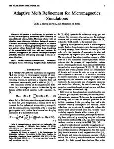
Indeed, for any CFD simulation, the boundary treatment is important in order to get accurate and reliable results. As mentioned earlier, the k − ω SST model is a blend of the k − ε and the k − ω with some additional features. One reason for this is that the k − ω model shows great sensitivity to the free stream values of ω whereas it behaves much better in the near wall regions than the k − ε model [1]. In addition to this, advanced wall treatment for ω has also been developed in order to make it less sensitive to near wall grid resolution, see [1] and [4]. To investigate how the new turbulence model performs, a test case was chosen to be airfoil simulations. The boundary conditions for this type of simulation can vary dependent on under which setting the airfoil is simulated. For example if it is present in a turbulent flow field or not affects the boundary conditions on k and ω and also, if large turbulent fluctuations approach the airfoil, the velocity as well. Below the boundary conditions applied in OpenFOAM are presented and discussed in connection to a typical computational domain as presented in Figure 2.1.

(a) Entire domain.

(b) Wing Patch.

Figure 2.1: Computational domain including patch names for NACA 4412 Airfoil.

The following table lists the boundary conditions applied in a two dimensional case.

7

2.2. BOUNDARY CONDITIONS

CHAPTER 2. THEORY

Table 2.1: Boundary conditions for the k − ω SST DES model.

Field U

p

k

ω

νt /νsgs

Patch Inlet Outlet Top Bottom Wing Inlet Outlet Top Bottom Wing Inlet Outlet Top Bottom Wing Inlet Outlet Top Bottom Wing Inlet Outlet Top Bottom Wing

Type freestream freestream freestream freestream fixedValue freestreamPressure freestreamPressure freestreamPressure freestreamPressure zeroGradient fixedValue zeroGradient fixedValue fixedValue fixedValue fixedValue zeroGradient fixedValue fixedValue omegaWallFunction calculated calculated calculated calculated fixedValue

Specifications freestreamValue freestreamValue freestreamValue freestreamValue uniform (0 0 0)

uniform uniform uniform uniform

(-1 (-1 (-1 (-1

0 0 0 0

0) 0) 0) 0)

uniform 1e-6 uniform uniform uniform uniform

1e-6 1e-6 1e-10 1

uniform uniform uniform uniform uniform uniform uniform uniform

1 1 1e3 0 0 0 0 0

In general, the boundary conditions are selected to simulate a case where the airfoil is traveling through a completely still fluid where no turbulence is present. One specific thing that is of great importance to achieve this is to set k and ω at the boundary such that the turbulent viscosity becomes small in comparison to the kinematic one. This is achieved by noting that far away from walls, the turbulent viscosity is given by k/ω and hence the relation between the two quantities can be chosen such that νt /ν is small. In this case νt /ν = 0.1. Below follows a short description of the boundary conditions employed for the different quantities. Velocity, U To begin with, a no-slip condition is applied to the airfoil, which is realized with the fixedValue boundary condition. At the other boundaries, the freestream boundary condition is applied. It is applicable at boundaries of type patch or wall and is a derived boundary condition of type inletOutlet. This means that for every face of the patch, the boundary condition will be assigned dependent on the local flux. If the flux goes inside the domain, it will be assigned a fixed value and if it goes out it will be assigned a zero gradient condition. This is typically what we want to achieve in this case. Pressure, p The pressure boundary condition is of type zeroGradient on the wing. The physical motivation for this is that there is no flow through the wall and hence no pressure gradient should exist normal to the wall trying to drive the fluid through the wall. On the other boundaries, the boundary condition is of type freestreamPressure. The first thing to be noted here is that this boundary condition must be used together with the freestream boundary condition for U . It is applicable to boundaries of type patch or wall, and is a derived boundary condition of type zeroGradient. It sets what is known as a free-stream condition on the pressure. This means that it is a zero gradient condition that constrains the flux across the boundary based on the free stream velocity (U). 8

2.3. APPLYING RUN-TIME MESH REFINEMENT

CHAPTER 2. THEORY

Turbulent kinetic energy, k The turbulent kinetic energy is prescribed by setting it to a small value on the wing. What small means is really not well defined, so therefore it is good practice to simply prescribe it arbitrarily small and check that the simulations look reasonable. In reality, k = 0 on the wing since no turbulent fluctuations are present at the wing. However some turbulence models include division of k in the transport equations and therefore it is better practice to choose k 6= 0. Note that no wall function approach is used, and hence the first internal grid point must be located at y + ≤ 11.63 [5]. On the inlet, top and bottom, it has simply been prescribed to some arbitrary small number such that νt /ν = 0.1. A zero gradient condition is used at the outlet simply to not disturb the wake forming behind the airfoil. Turbulent frequency, ω On the wing, a special boundary condition has been applied to ω through omegaWallFunciton. The reason to use special wall functions is that ω → ∞ as y → 0, and hence it can not simply be specified at the wall. Instead it is set in the first internal node using a special formula. A version of this type of wall treatment is presented in [4], although it needs to be stated that this is not the exact same approach that is taken in OpenFOAM. The method applied in OpenFOAM is essentially a blend between the usual low-Re formulation and a wall function treatment dependent on if the grid is too coarse close to the wall. In short, ω is set in the first internal node as a squared average between the low-Re formulation and wall function formulation according to q 2 + ω2 . (2.15) ω = ωVis log Here ωVis and ωlog are computed according to

ωVis

=

ωlog

=

6ν , β1 y 2 √ k √ . 4 ∗ β κy

(2.16) (2.17)

This allows for a smooth mixing, that automatically sets a suitable value for ω in the first node dependent on its location. At the inlet, top and bottom, the values are prescribed in order for the turbulent/sub grid scale viscosity to be small in comparison to the kinematic viscosity and hence simulate little presence of turbulence. Turbulent viscosity/Sub grid scale viscosity, νt /νsgs On the wing, the turbulence goes to zero and hence any shear stresses caused by turbulence should be zero here as well. Therefore, the turbulent or sub grid scale, viscosity is set to zero at the wing. For the other boundaries, the calculated boundary condition is applied. This means that no special boundary condition is assigned to the turbulent viscosity, but it is assumed to have been assigned using other fields. This is appropriate since we want k and ω to determine νt /νsgs , but still some boundary condition needs to be applied since the turbulent viscosity is needed in the 0/ directory.

2.3

Applying run-time mesh refinement

In this project, mesh refinement is also going to be used. Since the mesh refinement should happen automatically at run-time, some quantity needs to exist that indicates if the mesh should be refined in a certain location. One way to do this, which is implemented in OpenFOAM, is to store a value for every cell and then refine a certain cell if the value lies within a specific interval. The limits and which type of scalar field that is used as an indicator is then up to the user to decide. In this project, the aim is to adapt the mesh such that turbulence is resolved. This means that if turbulence is resolved, the mesh does not need to be refined. However in regions where the turbulence exists, but its length scales are smaller than the local grid size, the mesh should be refined in order to resolve turbulence here. The natural way to achieve this is to work with the FDES or 9

2.3. APPLYING RUN-TIME MESH REFINEMENT

CHAPTER 2. THEORY

FDDES term, see (2.13) and (2.14). If this term is larger than 1, the DES effect has been enabled and the model should hopefully start to resolve turbulence in that region. On the other hand if it is equal to 1, the model operates in RANS mode in that region and no turbulence should be resolved. For the DES and DDES model, the ratio of the turbulent to the grid length scale is therefore defined as √

LDES

=

LDDES

=

k , CDES β ∗ ω∆ √ k (1 − FS ). CDES β ∗ ω∆

(2.18) (2.19)

Since these are the terms within the max operator in (2.13) and (2.14) respectively, it holds that the DES features are active if FDES or FDDES are greater than 1. To select the regions in which mesh refinement should be applied, this term is therefore going to be used as an indicator. If it is greater than some αu , it is sufficiently large and no mesh refinement is needed. On the other hand if it is less than some constant αl close to 0, we have a region in which very little turbulence is present and mesh refinement in unnecessary. If it however lies in between these two limits, we have a region in which turbulence is present but the mesh is not fine enough, or just about fine enough, to resolve turbulence. Here mesh refinement is appropriate. Hence a good indicator of mesh refinement is that αl ≤ FDES ≤ αu or αl ≤ FDDES ≤ αu depending on the model used. The lower and upper limit must be tuned by repeated simulations and evaluation of results.

10

Chapter 3

The OpenFOAM implementation In this chapter the implementation of a LES-class turbulence model, namely the k − ω SST SAS model, as well as the dynamic mesh features of the pimpleDyMFoam solver are described. The reason that the k − ω SST SAS model will be described is that it will later be modified into the k − ω SST DES model as mentioned in the introduction. The discussion does mainly regard high level programming and technical details on a deeper level are left out. The aim is to give a general understanding of the implementation in order to be able to modify the turbulence model as well as using the dynamic mesh features of the solver.

3.1

k − ω SST SAS model

The declaration and definition files of the k − ω SST SAS turbulence model are found at $FOAM_SRC / turbulenceModels / incompressible / LES / kOmegaSSTSAS /

3.1.1

kOmegaSSTSAS.H

The declaration file kOmegaSSTSAS.H is presented in parts below. It begins by including some declaration files before the class declaration starts, as seen below. 55 56 57 58 59 60 61 62 63 64 65 66 67 68 69 70 71 72 73 74

# ifndef kOmegaSSTSAS_H # define kOmegaSSTSAS_H # include " LESModel . H " # include " volFields . H " # include " wallDist . H " // * * * * * * * * * * * * * * * * * * * * * * * * * * * * * * * * // namespace Foam { namespace incompressible { namespace LESModels { /* - - - - - - - - - - - - - - - - - - - - - - - - - - - - - - - - - - - - - - - - - - - - - - - - - - - - - - - - - - - - - - - - -*\ Class kOmegaSSTSAS Declaration \* - - - - - - - - - - - - - - - - - - - - - - - - - - - - - - - - - - - - - - - - - - - - - - - - - - - - - - - - - - - - - - - - - */ 11

3.1. K − ω SST SAS MODEL

75 76 77 78 79 80 81 82 83 84 85 86 87 88 89 90 91 92 93 94 95 96 97 98 99 100

CHAPTER 3. THE OPENFOAM IMPLEMENTATION

class kOmegaSSTSAS : public LESModel { // Private Member Functions // - Update sub - grid scale fields void u p d a t e S u b G r i d S c a l e F i e l d s ( const volScalarField & D ); // Disallow default bitwise copy construct and assignment kOmegaSSTSAS ( const kOmegaSSTSAS &); kOmegaSSTSAS & operator =( const kOmegaSSTSAS &);

protected : // Protected data // Model constants dime nsione dScal ar alphaK1_ ; dime nsione dScal ar alphaK2_ ; dime nsione dScal ar alphaOmega1_ ; dime nsion edScal ar alphaOmega2_ ; Listing 3.1: file: kOmegaSSTSAS.H

To save some space, a set of model constant declarations have been left out. After them, the declaration of the fields the model uses and calculates follows. 124 125 126 127 128 129

// Fields volScalarField k_ ; volScalarField omega_ ; volScalarField nuSgs_ ; Listing 3.2: file: kOmegaSSTSAS.H

To begin with there is the declaration files. LESModel.H is included since this turbulence model inherits the LESModel class and hence is a sub class to this class. Furthermore, wallDist.H is included to enable the calculation of distance to walls, as the name indicates. It uses the utility patchDist, but only calculates the distance to boundaries of type wall, not a general patch. This allows the user to select which boundaries that the solver should actually interpret as physical walls and not as general boundaries such as an inlet or cyclic patch. For more details on wallDist and patchDist, please refer to the installation where they are found at $FOAM_SRC / finiteVolume / fvMesh / wallDist / After the declaration files, the namespace is set for this turbulence model, and as seen all declarations and so forth will be done in namespace Foam::incompressible::LESModel. Hence functions used in this turbulence model will be those developed for incompressible LES models. Next, starting on line 76. the class is declared, and as seen it also inherits the attributes of the LESModel class and thus becomes a sub class to LESModel. Next follows a set of declarations, first of updateSubgridScaleFields, which is a function updating the turbulent/subgrid scale viscosity 12



using call-by-reference. Since it does not say public: or protected: above we also know that this is a private member function. After this a set of member constants and member fields are declared. They are set as protected, meaning that they are visible only within this class and classes that inherit from the class kOmegaSSTSAS as well as friend functions to this class. Also when run-time mesh refinement is used, a separate field depicting where mesh refinement should occur is needed as well. For this purpose a new volScalarField will have to be added as well. The model constants that the SAS and DES implementation share have the same values in both models. The only difference is that the models use some specific constants in their respective source terms. It should also be mentioned that the names used in this implementation differ to some extent from the names found in [2]. When describing how to do the DES implementation, the corresponding names in literature and implementation will be presented to avoid confusion. Next the protected member functions are declared, the first one are shown below 131 132 133 134 135 136 137 138 139 140 141 142 143 144 145 146 147 148 149 150 151 152 153 154 155 156 157 158

// Protected Member Functions tmp < volScalarField > Lvk2 ( const volScalarField & S2 ) const ; tmp < volScalarField > F1 ( const volScalarField & CDkOmega ) const ; tmp < volScalarField > F2 () const ; tmp < volScalarField > blend ( const volScalarField & F1 , const dimens ionedS calar & psi1 , const dimens ionedS calar & psi2 ) const { return F1 *( psi1 - psi2 ) + psi2 ; } tmp < volScalarField > alphaK ( const volScalarField & F1 ) const { return blend ( F1 , alphaK1_ , alphaK2_ ); } Listing 3.3: file: kOmegaSSTSAS.H

These protected functions will only be visible in the same way as for the protected member data shown above. Here, typically, different functions needed to evaluate complex terms within the transport equations as well as blending functions used to shift between the model formulations are declared. It is generally more convenient to define functions returning these terms, than to state them explicitly when setting up and discretizing the transport equations. When modifying the turbulence model, the FDES or FDDES should also be declared here. It is worth noting that all these functions return volScalarFields (related to the mesh), but they are also of class tmp. The wrapper class tmp is used for large objects (memory wise) and allows them to be returned from the function without being copied. It also allows the memory occupied by this object to be cleared as soon as it is not used anymore. In short, it is the function type of choice when calculating and

13



returning large fields that will only be used temporarily to compute some term or quantity in the transport equations. Furthermore, the keyword const is predominantly used throughout member function declarations above. The second const, used after defining which parameters to take in, says that this function may not modify the original objects it takes in. The first ones says that the object sent in is of type constant. The function blend is also defined here, not just declared. It is the implementation of (2.7) and (2.8) and is used to blend the model constants. The reason to why only one type of blend function is needed is that the values of 1/σkj and 1/σωj are used instead of σkj and σωj . An example of how blend is applied is seen in the next member function, where 1/σk is computed using the blending between the k − ω and the k − ε values. As can be seen the model constants do not have the same name in the implementation as in the papers it is based upon. Finally some public member functions are declared, the first piece of the code doing this is shown below 208 209 210 211 212 213 214 215 216 217 218 219 220 221

// Member Functions // - Return SGS kinetic energy virtual tmp < volScalarField > k () const { return k_ ; } // - Return omega virtual tmp < volScalarField > omega () const { return omega_ ; } Listing 3.4: file: kOmegaSSTSAS.H

The public member functions are visible outside of the class, and thus are typically functions returning fields that are of interest outside the turbulence model, such as k or ω. They are also virtual, meaning that their function are determined run-time.

3.1.2

kOmegaSSTSAS.C

The main definition file is presented in parts below. First comes some include files as well as the definition of the correct namespace and and the protected member functions 25 26 27 28 29 30 31 32 33 34 35 36 37 38 39 40

# include " kOmegaSSTSAS . H " # include " a d d T o R u n T i m e S e l e c t i o n T a b l e . H " # include " wallDist . H " // * * * * * * * * * * * * * * * * * * * * * * * * * * * * * * * * // namespace Foam { namespace incompressible { namespace LESModels { // * * * * * * * * * * * Static Data Members * * * * * * * * * * * //

14


41 42 43 44 45 46 47 48 49 50


d e f i n e T y p e N a m e A n d D e b u g ( kOmegaSSTSAS , 0); a d d T o R u n T i m e S e l e c t i o n T a b l e ( LESModel , kOmegaSSTSAS , dictionary ); // * * * * * * * * * Protected Member Functions * * * * * * * * * // void kOmegaSSTSAS :: u p d a t e S u b G r i d S c a l e F i e l d s ( const volScalarField & S2 ) { nuSgs_ == a1_ * k_ / max ( a1_ * omega_ , F2 ()* sqrt ( S2 )); nuSgs_ . c o r r e c t B o u n d a r y C o n d i t i o n s (); } Listing 3.5: file: kOmegaSSTSAS.C

To begin with, the previously considered declaration files kOmegaSSTSAS.H and wallDist.H are included. In this part we will see the use of the wall distance when it comes to calculating the different terms in the transport equations. The first protected member function is the one that computes the turbulent, or sub grid scale viscosity, called updateSubGridScaleFields. As can be noted, it is the exact same expression as (2.10) assuming that what is called S2 is equal to S 2 = 2¯ sij s¯ij . At line 348 this field is computed as 348

volScalarField S2 (2.0* magSqr ( symm ( gradU ()))); Listing 3.6: file: kOmegaSSTSAS.C

The programmers guide [6], section 1.4.1 gives, since gradU() simply gives the gradient of the vector field, that 1 ∇U + (∇U )T . 2 Furthermore, section 1.3.6 and 1.4.1 of the programmers guide gives that the magSqr operation performs a double inner product to a second order tensor according to symm(gradU()) =

magSqr(T) = T : T. From the programmers guide, section 1.3.2, we have that T : T = Tij Tij , where Tij are the components of the second order tensor. Hence, the implementation computes S2 as 1 ∂u ¯i ¯i ∂u ¯j 1 ∂ u ∂u ¯j S2 = 2 + + 2 ∂xj ∂xi 2 ∂xj ∂xi = 2¯ sij s¯ij . The second equality comes from definition (2.5). The conclusion is that the implementation uses the same formula for the turbulent/sub grid scale viscosity given in (2.10). Next the two blending functions F1 and F2 are defined 52 53 54 55 56 57 58 59 60 61 62 63

tmp < volScalarField > kOmegaSSTSAS :: F1 ( const volScalarField & CDkOmega ) const { tmp < volScalarField > CDkOmegaPlus = max ( CDkOmega , dim ension edScal ar ( " 1.0 e -10 " , dimless / sqr ( dimTime ) , 1.0 e -10) ); tmp < volScalarField > arg1 = min ( min 15


64 65 66 67 68 69 70 71 72 73 74 75 76 77 78 79 80 81 82 83 84 85 86 87 88 89 90 91 92


( max ( ( scalar (1)/ betaStar_ )* sqrt ( k_ )/( omega_ * y_ ) , scalar (500)* nu ()/( sqr ( y_ )* omega_ ) ), (4* alphaOmega2_ )* k_ /( CDkOmegaPlus * sqr ( y_ )) ), scalar (10) ); return tanh ( pow4 ( arg1 )); }

tmp < volScalarField > kOmegaSSTSAS :: F2 () const { tmp < volScalarField > arg2 = min ( max ( ( scalar (2)/ betaStar_ )* sqrt ( k_ )/( omega_ * y_ ) , scalar (500)* nu ()/( sqr ( y_ )* omega_ ) ), scalar (100) ); return tanh ( sqr ( arg2 )); } Listing 3.7: file: kOmegaSSTSAS.C

The implementation of these two blending functions differs slightly from formulas (2.6) and (2.11). In both cases there is an extra min(a, b) operation being performed in order to evaluate ξ and η (denoted arg1 and arg2) which then will go into the tanh function. For the case of F1 , the implementation instead computes the quantity tanh(ξ˜4 ), where ξ˜ = min(ξ, 10). The reason why is simply that tanh(104 ) is so close to 1, that any larger value of ξ than 10 simply does not affect the value of tanh to anything but a very small extent. Hence the implementation avoids forcing OpenFOAM to calculate tanh of some very large value of ξ 4 , hopefully giving a faster and/or more stable code. The analogous approach is used for F2 . Keeping this small change in mind, a look at the implementation reveals that it would be the same as the formulas (2.6) and (2.11) if it holds that CDkOmega = 2σω2

1 ∂k ∂ω . ω ∂xi ∂xi

At line 354 this term is calculated according to 354

volScalarField CDkOmega ((2.0* alphaOmega2_ )*( gradK & gradOmega )/ omega_ ); Listing 3.8: file: kOmegaSSTSAS.C

The & is an inner product in OpenFOAM, which for the vectors gradK and gradOmega gives the formula ∇k · ∇ω =

16

∂k ∂ω . ∂xi ∂xi



Hence the implementation uses the desired formula for the cross diffusion term as given in (2.9). The rest of the implemented protected member functions are specific to the SAS model. When adding the new FDES or FDDES term later on, it will be convenient to include it as a function like F1. This will make it easy to modify and view its implementation as well as switching between the DES and DDES formulation. Later on a volScalarField can then be created using this function, prior to setting up and solving the discrete system of equations. Next comes the construction of the object kOmegaSSTSAS 116 117 118 119 120 121 122 123 124 125 126 127 128 129 130 131 132 133 134 135 136 137 138 139 140 141 142 143 144 145 146 147

// * * * * * * * * * * * * * Constructors

* * * * * * * * * * * * //

kOmegaSSTSAS :: kOmegaSSTSAS ( const volVectorField & U , const su rf ac eS ca la rF ie ld & phi , transportModel & transport , const word & turbulenceModelName , const word & modelName ) : LESModel ( modelName , U , phi , transport , tu r b ul e n ce M o de l N am e ) , alphaK1_ ( dimensioned < scalar >:: l ookupO rAddTo Dict ( " alphaK1 " , coeffDict_ , 0.85034 ) ), alphaK2_ ( dimensioned < scalar >:: l ookupO rAddTo Dict ( " alphaK2 " , coeffDict_ , 1.0 ) ), Listing 3.9: file: kOmegaSSTSAS.C

To save some space, not all definitions of protected member constants have been included. They are followed by the fields used by the turbulence model as follows. 286 287 288 289 290 291 292 293 294 295

k_ ( IOobject ( "k", runTime_ . timeName () , mesh_ , IOobject :: MUST_READ , IOobject :: AUTO_WRITE 17


296 297 298 299 300 301 302 303 304 305 306 307 308 309 310 311 312 313 314 315 316 317 318 319 320 321 322 323 324 325 326 327 328 329 330 331 332 333 334


), mesh_ ), omega_ ( IOobject ( " omega " , runTime_ . timeName () , mesh_ , IOobject :: MUST_READ , IOobject :: AUTO_WRITE ), mesh_ ), nuSgs_ ( IOobject ( " nuSgs " , runTime_ . timeName () , mesh_ , IOobject :: MUST_READ , IOobject :: AUTO_WRITE ), mesh_ ) { omegaMin_ . readIfPresent (* this ); bound ( k_ , kMin_ ); bound ( omega_ , omegaMin_ ); u p d a t e S u b G r i d S c a l e F i e l d s (2.0* magSqr ( symm ( fvc :: grad ( U )))); printCoeffs (); } Listing 3.10: file: kOmegaSSTSAS.C

After the appropriate parameters have been taken in to construct the object kOmegaSSTSAS, the construction begins by directly calling the constructor of the LESModel class. After this all model constants are read from a sub dictionary in the LESProperties dictionary called kOmegaSSTSASCoeffs, or defined if not present. Also all the relevant fields, such as k and ω are read. Since the DES model includes a new model constant, it is important to include it here as well. Also, in the case of run-time mesh refinement, a new field is needed which will be computed by the turbulence model. Thus it must also be read here in order to be computed. The maybe most important thing in the body of the constructor is the call for the calculation of the turbulent viscosity through the function updateSubGridScaleFields. The final part of the turbulence model includes solving for the turbulent quantities k and ω together with the calculation of νt /νsgs . This is done in the virtual void function correct, which is a public member function of the class kOmegaSSTSAS as can be seen in the declaration file kOmegaSSTSAS.H. Hence, since it is a virtual function, it will override the function correct in 18



the LESModel class, which the kOmegaSSTSAS class inherited. This allows OpenFOAM to select which turbulence model that is used run-time, since the function calculating the turbulent viscosity is overridden by the chosen turbulence model. It starts by solving the equation for k 336 337 338 339 340 341 342 343 344 345 346 347 348 349 350 351 352 353 354 355 356 357 358 359 360 361 362 363 364 365 366 367 368 369 370 371 372 373 374 375 376 377 378 379

// * * * * * * * * * * * * Member Functions

* * * * * * * * * * * //

void kOmegaSSTSAS :: correct ( const tmp < volTensorField >& gradU ) { LESModel :: correct ( gradU ); if ( mesh_ . changing ()) { y_ . correct (); } volScalarField S2 (2.0* magSqr ( symm ( gradU ()))); gradU . clear (); volVectorField volVectorField volScalarField volScalarField volScalarField volScalarField

gradK ( fvc :: grad ( k_ )); gradOmega ( fvc :: grad ( omega_ )); L ( sqrt ( k_ )/( pow025 ( Cmu_ )* omega_ )); CDkOmega ((2.0* alphaOmega2_ )*( gradK & gradOmega )/ omega_ ); F1 ( this - > F1 ( CDkOmega )); G ( GName () , nuSgs_ * S2 );

// Turbulent kinetic energy equation { fvScalarMatrix kEqn ( fvm :: ddt ( k_ ) + fvm :: div ( phi () , k_ ) - fvm :: laplacian ( DkEff ( F1 ) , k_ ) == min (G , c1_ * betaStar_ * k_ * omega_ ) - fvm :: Sp ( betaStar_ * omega_ , k_ ) ); kEqn . relax (); kEqn . solve (); } bound ( k_ , kMin_ ); tmp < volScalarField > grad_omega_k = max ( magSqr ( gradOmega )/ sqr ( omega_ ) , magSqr ( gradK )/ sqr ( k_ ) ); Listing 3.11: file: kOmegaSSTSAS.C

What can first be noted is that support for a changing mesh is included, in which case the wall distance will be corrected by letting the function correct() operate on the field. After this a set of fields necessary to set up the discrete system of equations are calculated. Since the names of the different operations are very logical in OpenFOAM, it is not necessary to explain all of these

19



fields. The fields S2 and CDkOmega have already been considered, and the only one that raises some questions is the field called G. This is the production term Pk without the limiter applied to it, since according to the implementation we have G

=

νt S 2

= νt 2¯ sij s¯ij ¯ ij 2νt s¯ij s¯ij + Ω u ¯j 1 ∂u ¯i ∂u ¯j 1 ∂u ¯i ∂u ¯j ∂u ¯i + + + − = νt ∂xj ∂xi 2 ∂xj ∂xi 2 ∂xj ∂xi ∂u ¯i u ¯j ∂u ¯i = νt + ∂xj ∂xi ∂xj = Pk . =

¯ ij and the symmetric tensor s¯ij is Here it was used that the product of the anti symmetric tensor Ω ¯ ij = −Ω ¯ ji . zero since Ω When implementing the DES model it is the dissipation in the k equation that will be modified by multiplying it with an extra term, namely FDES or FDDES . This field must also be calculated in advance using the function describing it. Turning to the creation of the discrete system of equations, the transport equation for k is set up in accordance with (2.2) apart from the fact that no DES term is included. The production term can be seen to include the limiter, as written in (2.12) since c1 = 10. Further the dissipation term comes in by using the operation fvm::Sp(betaStar *omega , k ). Indeed the dissipation term could simply have been added by writing betaStar *omega *k , in which case it would have been implemented explicitly. The thing is though that the entire dissipation term always is negative due to the minus sign, and the fact that k, ω and β∗ are positive. To improve convergence and stability it is better to treat negative sources implicitly, which is achieved using the syntax Sp(). The answer to why is because when a source term is treated explicitly, it is included in the load vector b in the discretisized system of equations Ak = b, where k is a vector including the nodal values of k. Hence it can prior to convergence cause the elements in k to go negative, which is bad when considering that k ≥ 0 by definition. However, when it is treated implicitly, it is instead included in the diagonal of A instead. Since it was negative on the right hand side, it will instead give a positive contribution on the left hand side, making the matrix A more diagonally dominant. After the k equation has been solved, the ω equation is set up and solved according to 380 381 382 383 384 385 386 387 388 389 390 391 392 393 394 395 396 397 398

// Turbulent frequency equation { fvScalarMatrix omegaEqn ( fvm :: ddt ( omega_ ) + fvm :: div ( phi () , omega_ ) - fvm :: laplacian ( DomegaEff ( F1 ) , omega_ ) == gamma ( F1 )* S2 - fvm :: Sp ( beta ( F1 )* omega_ , omega_ ) - fvm :: SuSp // cross diffusion term ( ( F1 - scalar (1))* CDkOmega / omega_ , omega_ ) + FSAS_ * max ( 20

3.2. PIMPLEDYMFOAM

399 400 401 402 403 404 405 406 407 408 409 410 411


dime nsione dScala r ( " zero " , dimensionSet (0 , 0 , -2 , 0 , 0) , 0.0) , zetaTilda2_ * kappa_ * S2 * sqr ( L / Lvk2 ( S2 )) - 2.0/ alphaPhi_ * k_ * grad_omega_k ) ); omegaEqn . relax (); omegaEqn . solve (); } bound ( omega_ , omegaMin_ ); u p d a t e S u b G r i d S c a l e F i e l d s ( S2 ); } Listing 3.12: file: kOmegaSSTSAS.C

The implementation is the same as presented in (2.3) apart from the so called SAS term, which of course must be removed when implementing the DES model. Another interesting thing that can be noted here is the implementation of the cross diffusion term according to fvm::SuSp(F1 scalar(1)*CDkOmega/omega , omega ). The use of SuSp(a,b) allows for a flexible treatment of the source term with respect to the sign of a. If it is negative, the source term is treated implicitly, and if it is positive it will be treated explicitly. Explicit treatment is favorable if the source term is positive and hence it will be done if possible. Finally it can be seen that the turbulent viscosity is updated, and hence the purpose of the correct function is achieved in a sense. When a new field for mesh refinement is added, it will be calculated here as well, using the most recent values of k and ω. The final thing that should be reviewed in order to be able to implement the DES model is the name and the values of the model constants. As it turns out, their names in the implementation do not always correspond to the literature. The following table presents the names and values used in the implementation, together with the corresponding names used in the literature. Table 3.1: Model constant names used in implementation and corresponding names in theory.

Theory α1 α2 β1 β2 1/σk1 1/σk2 1/σω1 1/σω2 β∗ a1 CDES

3.2

Implementation gamma1 gamma2 beta1 beta2 alphaK1 alphaK2 alphaOmega1 alphaOmega2 betaStar a1 CDES

Value in implementation 0.5532 0.4403 0.075 0.0828 0.85034 1.0 0.5 0.85616 0.09 0.31 0.61

pimpleDyMFoam

The solver pimpleDyMFoam is a modification of the pimpleFoam solver that supports meshes of class dynamicFvMesh. The class dynamicFvMesh is a base class for meshes that can move and/or change topology. The solver pimpleFoam is a transient solver developed for incompressible flows, and is based on the PISO and SIMPLE algorithms. It is in addition to the pisoFoam solver, which is based on the PISO algorithm, developed to be able to handle larger time steps. This section will not focus on how the actual transport equations are solved using the merged PISO-SIMPLE algorithm, but on

21

3.2. PIMPLEDYMFOAM


how the dynamic meshes are treated within the solver. There are a number of different sub classes to the class dynamicFvMesh, based upon what the mesh should be able to do. Since pimpleDyMFoam primarily is developed for moving meshes, special attention will also be paid towards how this solver will treat a refined mesh and if there are missing features left to be implemented for this purpose. The pimpleDyMFoam solver is located at $FOAM_APP / applications / solvers / incompressible / pimpleFoam /\ pimpleDyMFoam / Furthermore, for reference, the pimpleFoam solver are located at $FOAM_APP / applications / solvers / incompressible / pimpleFoam /

3.2.1

Comparison between pimpleFoam.C and pimpleDyMFoam.C

To begin with the differences in the definition files of the original pimpleFoam solver and the pimpleDyMFoam solver will be presented. The pimple-loop, in which both solvers solve the transport equations, are essentially equal. Some differences are present to handle mesh movement in the pimpleDyMFoam case but otherwise they are the same. The major differences are instead present before the pimple-loop. Everything before the pimple-loop, excluding the header, is presented for the pimpleFoam.C file below. 36 37 38 39 40 41 42 43 44 45 46 47 48 49 50 51 52 53 54 55 56 57 58 59 60 61 62 63 64 65 66 67 68

# include # include # include # include # include # include # include

" fvCFD . H " " singlePhaseTransportModel .H" " turbulenceModel . H " " pimpleControl . H " " fvIOoptionList . H " " I O p or o s it y M od e l Li s t . H " " IOMRFZoneList . H "

// * * * * * * * * * * * * * * * * * * * * * * * * * * * * * * * * // int main ( int { # include # include # include # include # include # include

argc , char * argv []) " setRootCase . H " " createTime . H " " createMesh . H " " createFields . H " " createFvOptions . H " " in it Co nt in ui ty Er rs . H "

pimpleControl pimple ( mesh ); // * * * * * * * * * * * * * * * * * * * * * * * * * * * * * * // Info < < " \ nStarting time loop \ n " FDES ()); volScalarField FDDES ( this - > FDDES ( F1 )); Listing 4.14: file: kOmegaSSTDES.C

Once again, note that it is the DDES features that are implemented here. Also note that it is crucial that the FDDES is computed after the F1 field, since it relies on it as a parameter. Next the transport equation for k is going to be modified so that the dissipation term includes the DES modification. This is done by adding the newly computed field FDES or FDDES into the first slot of the Sp( , ) function creating the source term. The final result should look like // Turbulent kinetic energy equation { fvScalarMatrix kEqn ( fvm :: ddt ( k_ ) + fvm :: div ( phi () , k_ ) 39

4.1. K − ω SST DES

CHAPTER 4. IMPLEMENTING K − ω SST DES

- fvm :: laplacian ( DkEff ( F1 ) , k_ ) == min (G , c1_ * betaStar_ * k_ * omega_ ) - fvm :: Sp ( betaStar_ * FDDES * omega_ , k_ ) // - fvm :: Sp ( betaStar_ * FDES * omega_ , k_ )

// F_DDES modification // F_DES modification

); Listing 4.15: file: kOmegaSSTDES.C

Note that it does not work to include the FDES/FDDES term in the second slot, i.e. multiplying it with k . After the k equation has been solved, a field unique to the SAS implementation is being calculated which is needed in a source term in the ω equation that is not used in the DES model. This field is called grad omega k and should be commented away according to /* tmp < volScalarField > grad_omega_k = max ( magSqr ( gradOmega )/ sqr ( omega_ ) , magSqr ( gradK )/ sqr ( k_ ) ); */ Listing 4.16: file: kOmegaSSTDES.C

The next thing that needs to be done is to remove the source term in the ω equation that is unique to the SAS model. It is the last entity of the equation and should be commented away to get the following // Turbulent frequency equation { fvScalarMatrix omegaEqn ( fvm :: ddt ( omega_ ) + fvm :: div ( phi () , omega_ ) - fvm :: laplacian ( DomegaEff ( F1 ) , omega_ ) == gamma ( F1 )* S2 - fvm :: Sp ( beta ( F1 )* omega_ , omega_ ) - fvm :: SuSp // cross diffusion term ( ( F1 - scalar (1))* CDkOmega / omega_ , omega_ ) /* + FSAS_ * max ( dime nsione dScala r (" zero " , dimensionSet (0 , 0 , -2 , 0 , 0) , 0.0) , zetaTilda2_ * kappa_ * S2 * sqr ( L / Lvk2 ( S2 )) - 2.0/ alphaPhi_ * k_ * grad_omega_k ) */ );

40

4.2. K − ω SST DES REFINE


Listing 4.17: file: kOmegaSSTDES.C

Finally, the read() function should be modified in order to exclude SAS model constants and include the new DES model constant. The read() function is present at the end of the file and should be modified according to bool kOmegaSSTDES :: read () { if ( LESModel :: read ()) { alphaK1_ . readIfPresent ( coeffDict ()); alphaK2_ . readIfPresent ( coeffDict ()); alphaOmega1_ . readIfPresent ( coeffDict ()); alphaOmega2_ . readIfPresent ( coeffDict ()); gamma1_ . readIfPresent ( coeffDict ()); gamma2_ . readIfPresent ( coeffDict ()); beta1_ . readIfPresent ( coeffDict ()); beta2_ . readIfPresent ( coeffDict ()); betaStar_ . readIfPresent ( coeffDict ()); a1_ . readIfPresent ( coeffDict ()); c1_ . readIfPresent ( coeffDict ()); // Cs_ . readIfPresent ( coeffDict ()); // alphaPhi_ . readIfPresent ( coeffDict ()); // zetaTilda2_ . readIfPresent ( coeffDict ()); // FSAS_ . readIfPresent ( coeffDict ()); CDES_ . readIfPresent ( coeffDict ()); omegaMin_ . readIfPresent (* this ); return true ; } else { return false ; } } Listing 4.18: file: kOmegaSSTDES.C

This concludes the modification of the turbulence model. The final thing to be done is to remove the kOmegaSSTDES.dep file and then recompile (wclean and then wmake libso). Therefore save and close the editor and then move into the directory where the Make and kOmegaSSTDES directories are situated. Then simply type wclean wmake libso This should build a new dynamic library including the new turbulence model. It will then be possible to link to this library and run simulations using the new turbulence model.

4.2

k − ω SST DES Refine

This section shows how to modify the k − ω SST DES turbulence model implemented above to work with the dynamic mesh refinement features of OpenFOAM. As previously discussed, the mesh 41



refinement needs a field to determine where the mesh should be refined and not. This field should be located in the time directory and hence must be computed, either by defining a function in the turbulence model or in the solver. This field will be a part of the FDES term of the turbulence model and hence the creation and output of this field is what is going to be added to the turbulence model. Before doing this, it should be stressed that the method shown here most certainly is not the only way to achieve this. The way it will be done is pretty straight forward, and follows the way the turbulent/sub grid scale viscosity is being computed and sent back. It was determined to not use the new field to further compute the FDES term, even though it is a part of it. Instead this part of the FDES term will be recomputed and returned, only to be used to govern mesh refinement. There are two reasons for this. The first is that the term includes the mesh size ∆, which only is defined in the node of a cell. Hence, at the boundary, there is no definition of what ∆ should be and hence an appropriate boundary condition can be hard to derive. Since the term will reside in the time directory, some boundary conditions should be imposed and thus the solution would run the risk of being affected by these if this term was actually used to evaluate FDES /FDDES . Secondly, it was found more convenient to leave the previous implementation intact and just add new features.

4.2.1

Creating the class kOmegaSSTDESRefine

This entire guide assumes that the k − ω SST DES turbulence model already has been implemented according to above. Start by opening a new terminal window and type OF22x to initialize the OpenFOAM environment. Next change directory to where the user turbulence models are implemented cd $ W M _ P R O J E C T _ U S E R _ D I R / src / turbulenceModels / incompressible / LES / Copy the kOmegaSSTDES turbulence model directory into a new directory called kOmegaSSTDESRefine according to cp -r kOmegaSSTDES / kOm eg aS ST DE SR ef in e / Change directory to the new turbulence model, remove the old kOmegaSSTDES.dep file and change name of the two remaining files according to cd rm mv mv

k Om eg aS ST DE SR ef in e / kOmegaSSTDES . dep kOmegaSSTDES . C k Om eg aS ST DE SR ef in e . C kOmegaSSTDES . H k Om eg aS ST DE SR ef in e . H

Then substitute the line kOmegaSSTDES for kOmegaSSTDESRefine in both the files, which will change the name of the class. sed -i s / kOmegaSSTDES / kO me ga SS TD ESR ef in e / g kO me ga SS TD ES Ref in e . H sed -i s / kOmegaSSTDES / kO me ga SS TD ESR ef in e / g kO me ga SS TD ES Ref in e . C Finally the model will be added to the files file, in order to tell the compiler that a new turbulence model should be added to the dynamic library. Open it using for example gedit cd .. gedit Make / files and add the following line after the previous turbulence model k Ome ga SS TD ES Re fi ne / k Om ega SS TD ES Re fi ne . C Finally recompile the dynamic library and make sure that everything works 42



wclean wmake libso

4.2.2

Modifying kOmegaSSTDESRefine.H

We will start by going back into the directory where the new turbulence is situated and open it cd $ W M _ P R O J E C T _ U S E R _ D I R / src / turbulenceModels / incompressible / LES /\ kO me ga SS TD ES Re fi ne / gedit kO me ga SS TD ES Re fi ne . H As for the previous model, add a small description and disclaimer in the beginning of the file, instead of the previous one according to Description k - Omega - SST - DES LES turbulence model for incompressible flows based on : " Ten Years of Industrial Experience with the SST Turbulence Model " . Turbulence Heat and Mass Transfer 4. F . R . Menter , M . Kuntz , R . Langtry . A note on the implementation with respect to the paper : - The transport equations implemented are divided by rho , as opposed to the presentation of them in the paper , since the flow is incompressible - There is a choice to use the model in DES ( Detached Eddy Simulation ) mode or DDES ( Delayed Detached Eddy Simulations ) mode . The latter protects the boundary layer from being resolved with LES and is used by default . The other part is commented away . - Model constants are not allways named the same as in the paper , see comments in declaration of constants below . - A extra volScalarField called LDES or LDDES ( dependent on which turbulence model that is used ) is calculated . It is not influencing the solution , but used solely as a field to indicate where the mesh needs refinement in order to resolve turbulence . The same quantity is used to calculate the F_DES or F_DDES term in the k equation , but this is done using a different routine . LDES = L_t /( C_DES * delta ) , LDDES = L_t /( C_DES * delta )*(1 - F_S ) ------------------------------------------------------------------------------DISCLAIMER : This is a student project work in the course CFD with OpenSource software taught by Hakan Nilsson , Chalmers University of Technology , Gothenburg , Sweden . ------------------------------------------------------------------------------Listing 4.19: file: kOmegaSSTDESRefine.H

Turning to the class declaration, a new void function calculating the term presented in (2.18) or (2.19) depending on turbulence model will be added. This will resemble the already existing function updateSubGridScaleFields which calculates the turbulent/sub grid scale viscosity. The new field will be denoted LDES or LDDES , where the first L is used to denote that it is a measure between two 43



different length scales, the turbulent one and the mesh. Add the following lines after the declaration of the function updateSubGridScaleFields // Calculate the LDES / LDDES fields // void updateLDES (); void updateLDDES ( const volScalarField & FS ); Listing 4.20: file: kOmegaSSTDESRefine.H

As for previous implementations, the DDES formulation is implemented and the DES formulation is commented away. Since a new field is introduced, it must also be declared. Therefore, add a declaration of the new field LDES or LDDES after the declaration of the k , omega and nuSgs fields and in front of the commented declaration of Lvk2 according to // Extra field to indicate mesh refinement // volScalarField LDES_ ; volScalarField LDDES_ ; Listing 4.21: file: kOmegaSSTDESRefine.H

This concludes the modifications needed to the declaration file.

4.2.3

Modifying kOmegaSSTDESRefine.C

To begin with, we will add the definition of the protected member function that computes LDES or LDDES defined in (2.18) and (2.19) respectively. To do this, add the following lines after the definition of updateSubGridScaleFields /* void kOm eg aS ST DE SR ef in e :: updateLDES () { LDES_ == sqrt ( k_ )/( CDES_ * betaStar_ * omega_ * delta ()); LDES_ . c o r r e c t B o u n d a r y C o n d i t i o n s (); } */ void kOm eg aS ST DE SR ef in e :: updateLDDES ( const volScalarField & FS ) { LDDES_ == sqrt ( k_ )/( CDES_ * betaStar_ * omega_ * delta ())*( scalar (1) - FS ); LDDES_ . c o r r e c t B o u n d a r y C o n d i t i o n s (); } Listing 4.22: file: kOmegaSSTDESRefine.C

Now that the function is defined, we must make sure that the new field, or object, is added in the construction of the class kOmegaSSTDESRefine. Therefore, add the construction of the fields LDES and LDDES after the construction of nuSgs field. Also, make sure to add an extra comma after the construction of nuSgs to obtain nuSgs_ ( IOobject 44



( " nuSgs " , runTime_ . timeName () , mesh_ , IOobject :: MUST_READ , IOobject :: AUTO_WRITE ), mesh_ ),

// Don ’t forget this comma !

/* LDES_ ( IOobject ( " LDES " , runTime_ . timeName () , mesh_ , IOobject :: MUST_READ , IOobject :: AUTO_WRITE ), mesh_ ) */ LDDES_ ( IOobject ( " LDDES " , runTime_ . timeName () , mesh_ , IOobject :: MUST_READ , IOobject :: AUTO_WRITE ), mesh_ ) Listing 4.23: file: kOmegaSSTDESRefine.C

As noted when kOmegaSSTSAS.C was considered, the turbulent/sub grid scale viscosity is computed inside the body of the constructor. This could of course be done for LDES or LDDES as well but there is no point in doing this. The reason is that the field is never used, only updated after k and ω have been solved for. Hence, it does not need to be calculated prior to solving for k and ω in contrast to the viscosity, which is needed for this purpose. The last modification is therefore to make sure that the new field is calculated using the newly calculated fields k and ω. For this purpose, add the following lines at the very end of the correct function after both k and ω have been solved for and the turbulent/sub grid scale viscosity have been updated using the function updateSubGridScaleFields // Update the LDES / LDDES term // updateLDES (); updateLDDES ( F1 ); Listing 4.24: file: kOmegaSSTDESRefine.C

45



This concludes the creation of the kOmegaSSTDESRefine model. After saving and closing, remove the kOmegaSSTDESRefine.dep file and then go to the directory containing the turbulence models and the Make directory and type wclean wmake libso This will rebuild the dynamic library containing the user defined turbulence models to include the new turbulence model kOmegaSSTDESRefine. Since this model will need a new field in the 0/ directory of a case that uses it, please refer to the tutorial section for a guide on how to add this as well.

46

Chapter 5

Simulation with mesh refinement This chapter describes how to set up a case to run airfoil simulations with mesh refinement. It requires that the reader has implemented the k − ω SST DES turbulence model for mesh refinement (kOmegaSSTDESRefine) according to the previous chapter. The case will be set up so that the solution can run in either 2 or 3D and with only the pimpleDyMFoam solver. For this purpose, a 2D mesh of a NACA 4412 airfoil, that is prepared for 3D simulations, have been supplied. At the end, the results of the simulation, both with respect to how the new turbulence model performs and to how the mesh refinement works, will be presented and briefly discussed.

5.1

Copying files

To begin with, a new OpenFOAM case will be created. Begin by creating a new case by copying an existing LES tutorial according to run cp -r $FOAM_TUTORIALS / incompressible / pisoFoam / les / pitzDaily . mv pitzDaily Ai rfoil4 412Ref ine cd Air foil4 412Ref ine Before modifying anything, we will also need a dynamicMeshDict for the pimpleDyMFoam solver. The interDyMFoam solver in OpenFOAM utilizes mesh refinement and hence a dictionary from one of the interDyMFoam tutorials will be copied into the constant directory. cp $FOAM_TUTORIALS / multiphase / interDyMFoam / ras / d a m B r e a k W i t h O b s t a c l e /\ constant / dynamicMeshDict constant / Proceed by removing the old blockMeshDict and the boundary file according to rm constant / polyMesh / blockMeshDict rm constant / polyMesh / boundary In the supplied files to this work, a file called blockMeshDict 4412 2D3D has been supplied. Copy this blockMeshDict into the constant/polyMesh/ directory. When this is done, rename it as well by typing mv constant / polyMesh / b l o c k M e s h D i c t _ 4 4 1 2 _ 2 D 3 D \ constant / polyMesh / blockMeshDict This blockMeshDict will by default give a 2D mesh (one cell in third direction) when running blockMesh. However, the front and back patches of the mesh are not of type empty, but instead of type cyclic. Hence, cyclic boundary conditions will also be prescribed on all flow fields, but if only one cell is present in the third direction the simulation will effectively be 2D. The reason for this is

47

5.2. CREATING THE MESH

CHAPTER 5. SIMULATION WITH MESH REFINEMENT

to allow the user to choose either to tun the case 2D and save simulation time, or full 3D to allow for more realistic turbulence to be resolved. To obtain a 3D mesh, the 2D mesh needs to be extruded. This can be accomplished with the utility extrudeMesh in OpenFOAM, which needs a dictionary. This dictionary is acquired by typing cp $FOAM_APP / utilities / mesh / generation / extrude / extrudeMesh /\ extrudeMeshDict system / This concludes the copying of all necessary files for the case. These will now be modified in the upcoming sections.

5.2

Creating the mesh

In this section, the mesh will be created and if desired, also extruded to 3D. Start by letting blockMesh creating the 2D mesh by typing blockMesh To be able to extrude the mesh to 3D, we will have to modify the extrudeMeshDict according to our mesh. Open the file with a preferred editor and make the following changes. 1. Comment away constructFrom patch and uncomment constructFrom mesh to obtain constructFrom mesh ; // constructFrom patch ; // constructFrom surface ; 2. Change the source case of the mesh that will be extruded to the current case to obtain sourceCase " ../ Airfo il4412 Refine " ; 3. Tell the extrudeMesh utility that it is the front patch that should be extruded. This will effectively just add a set of layers in the third direction, giving a 3D mesh. It is the sourcePatches and exposedPatchName that should be changed to front and back respectively to obtain sourcePatches ( front ); // If construct from patch : patch to use for back ( can be same as sourcePatch ) exposedPatchName back ; 4. The mesh will be extruded linearly in the third direction, therefore uncomment the linearNormal option for extrudeModel, and comment the other options (wedge). The changes should look like // - Linear extrusion in point - normal direction extrudeModel linearNormal ; // - Wedge extrusion . If nLayers is 1 assumes symmetry around plane . // extrudeModel wedge ; 5. The amount of layers added on the front is specified by nLayers. The new mesh will therefore contain nLayers + 1 cells in the third direction after extrusion. Specify this parameter to obtain the desired amount of cells, the author chose 10, according to nLayers

10;

48

5.3. THE 0/ DIRECTORY


6. Set the expansion ratio for the new layers added to 1.0 according to expansionRatio

1.0;

7. There are a lot of different ways extrudeMesh can operate on the mesh, requiring a lot of different coefficients to be specified for different cases. This extrusion only needs the coefficient specified within linearNormalCoeffs. Therefore, comment away all other ”...Coeffs” sub dictionaries and make sure that linearNormalCoeffs is uncommented according to li ne ar No rm al Co ef fs { thickness }

0.1;

Here, the thickness of the added layer was changed to 0.1 as well. The thickness refers to the total thickness of all the new layers added, and hence the thickness of one new layer is in the case of no expansion ration thickness/nLayers. The original mesh have a thickness of 0.01, which will hence be obtained for the added cells here as well. When this is done, a 3D mesh can be obtained by typing extrudeMesh

5.3

The 0/ directory

After the mesh has been created, it’s time to specify proper boundary and initial conditions for the velocity, pressure and turbulent quantities. As the mesh is created, the wing is oriented with it’s leading edge in the positive x direction and it’s low pressure side in the positive y direction as shown in Figure 2.1. The boundary conditions in Table 2.1 together with cyclic boundary conditions connecting the front and back patch will be implemented. Note that cyclic boundary conditions must be specified in the blockMeshDict as well, i.e. it must be specified that these patches are going to be connected through cyclic boundary conditions. To begin with we will change the name of some of the patches in the existing files to fit our mesh. Therefore type the following when standing inside the case directory. sed sed sed sed sed sed sed sed sed sed

-i -i -i -i -i -i -i -i -i -i

5.3.1

s / lowerWall / bottom / g 0/ U s / upperWall / top / g 0/ U s / lowerWall / bottom / g 0/ p s / upperWall / top / g 0/ p s / lowerWall / bottom / g 0/ k s / upperWall / top / g 0/ k s / lowerWall / bottom / g 0/ nuSgs s / upperWall / top / g 0/ nuSgs s / lowerWall / bottom / g 0/ nuTilda s / upperWall / top / g 0/ nuTilda

Velocity

The velocity is specified in the file 0/U. The velocity will be set to 1 m/s using the freestream boundary conditions. Begin by changing the initial value of the velocity to the following internalField

uniform ( -1 0 0);

The inlet, outlet, top and bottom patch should all have the same boundary conditions, according to 49



inlet { type freestream ; freestreamValue uniform ( -1 0 0); } After this, it is time to add the wing patch, at which a no slip boundary condition will be applied. Therefore, add the following lines after the last of the previous four boundary conditions. wing { type value

fixedValue ; uniform (0 0 0);

} Finally, it is time to add the front and back patch, for which cyclic boundary conditions will be applied. This is done by first removing the patch called frontAndBack and adding the following lines front { type }

cyclic ;

back { type

cyclic ;

} Finish by saving and closing the velocity file.

5.3.2

Pressure

The pressure is specified in the file 0/p. The pressure will be initialized to zero everywhere, and no modification is therefore needed to the initial conditions. Continue by changing the boundary conditions at the inlet, outlet, top and bottom to freestreamPressure, according to inlet { type }

f re es tr ea mP re ss ur e ;

The boundary condition for the wing is set to zero gradient by adding this patch wing { type

zeroGradient ;

} Finally the boundary cyclic boundary conditions needs to be added. Do this by removing the frontAndBack boundary condition and add the same lines as for the velocity. Finish by saving and closing the file.

5.3.3

Turbulent kinetic energy

The turbulent kinetic energy conditions are specified in 0/k. Begin by changing the initial condition to a very small number according to 50


internalField


uniform 1e -06;

Proceed by setting the initial condition at the inlet, top and bottom according to inlet { type value }

fixedValue ; uniform 1e -06;

The outlet should be of type zeroGradient, which means that it should be changed to outlet { type }

zeroGradient ;

At the wing the turbulence is in theory zero, but for numerical stability we will avoid this and just set it to something very small. Therefore add the following lines to specify the wing wing { type value

fixedValue ; uniform 1e -10;

// Avoid zero

} Proceed by removing the frontAndBack patch boundary conditions and add the same lines as for the previous quantities to achieve cyclic boundary conditions over the front and back patch. Save and close the file.

5.3.4

Turbulent frequency

There is no file for the turbulent frequency, instead we will change the name of the file 0/nuTilda. Begin by changing it’s name mv 0/ nuTilda 0/ omega The first modification that will be done to the file is to change the name of the object to omega, giving the following object

omega ;

Proceed by changing the unit of the field to 1/s and the initial value of the field to 1 according to dimensions

[0 0 -1 0 0 0 0];

internalField

uniform 1;

After this the boundary condition at the inlet, top and bottom should be changed to look like inlet { type value }

fixedValue ; uniform 1;

The outlet should be zeroGradient. Therefore, change this boundary condition to the same as for the turbulent kinetic energy. After this, the wing will be treated with a special wall function for the turbulent frequency. To use this add the following lines for the wing patch 51



wing { type Cmu kappa E beta1 value

om egaWal lFunct ion ; 0.09; 0.41; 9.8; 0.075; uniform 1000;

} Finally, remove the boundary condition for frontAndBack and add the cyclic boundary conditions in accordance with before. Save and close the file.

5.3.5

Turbulent/Sub grid scale viscosity

The turbulent/sub grid scale viscosity conditions is specified in the file 0/nuSgs. Begin by setting the initial value to 1e-6, corresponding to k/ω. internalField

uniform 1e -6;

Continue by changing the boundary conditions at the inlet, outlet, top and bottom to calculated according to inlet { type value }

calculated ; uniform 0;

At the wing, no turbulence is present, therefore add the following lines to prescribe the boundary condition at the wing wing { type value

fixedValue ; uniform 0;

} As always, finish by removing the frontAndBack patch boundary conditions and add those to achieve cyclic conditions. After this save and close the file.

5.3.6

LDES/LDDES

A field governing mesh refinement is also needed. It is called LDES or LDDES dependent on if the DES or DDES model is used as described earlier. In this case, it is assumed that the DDES model is used and hence the field LDDES will be added. To achieve this copy the nuSgs file, then change the name and dimension of the object according to cp 0/ nuSgs 0/ LDDES sed -i s / nuSgs / LDDES / g 0/ LDDES sed -i s /"0 2 -1"/"0 0 0"/ g 0/ LDDES After opening the file change the boundary condition at the inlet, outlet, top and bottom to zeroGradient to achieve

52

5.4. THE DICTIONARIES

inlet { type }


zeroGradient ;

The zeroGradient condition is used because at a patch, there is no definition of the cell size ∆. Hence, it is better to simply assume that it varies little in the normal direction to the patch instead. Also, this field is not used by the turbulence model as discussed earlier, so it’s value at a boundary is not important in that sense. At the wing, we however know that this field asymptotically must go to zero, due to that the turbulent kinetic energy does. Hence, it is safe to keep the same boundary conditions as for the turbulent/sub grid scale viscosity.

5.4

The dictionaries

The next step is to set up the necessary dictionaries. The dictionaries that will modified are controlDict, fvSolution, fvSchemes, LESProperties and dynamicMeshDict.

5.4.1

controlDict

We start by changing the name of the solver according to sed -i s / pisoFoam / pimpleDyMFoam / g system / controlDict The end time must also be modified. Before enabling mesh refinement, the flow must develop properly since we are dealing with a transient simulation. The wing is 1 m long the the flow is passing it at 1 m/s, so the end time will be chosen to 3 s in order to let the flow pass the wing several times. The change is done according to sed -i s /0.1/3/ g system / controlDict Further, change the ∆t value to 1 · 10−3 sed -i s /1 e -05/1 e -03/ g system / controlDict The write control should be set to adjustable, since the ∆t value will be governed by the Courant number, hence do the following change sed -i s / timeStep / a djusta bleRun Time / g system / controlDict The time intervals for which the solver will write out the results will be set next. The reader can of course choose this as they wish, for now it will be set to 0.2 s according to sed -i s /100/0.2/ g system / controlDict Let’s also change the purgeWrite option to only keep the latest solutions written and overwrite older. Here, this number will be changed to 5 sed -i s /" purgeWrite

0"/" purgeWrite

5"/ g system / controlDict

To save some space on the disc, especially in case of a 3D simulation in which the amount cells quickly become very large, write compression will be enabled sed -i s / off / compressed / g system / controlDict After this, open the file in an editor and add the following lines before the functions

53


adjustTimeStep

yes ;

maxCo

0.4;


libs (" l i b m y I n c o m p r e s s i b l e L E S M o d e l s . so "); This will enable run-time ∆t adjustment based on the Courant number, and also include the k − ω SST DES turbulence model. Furthermore, since the specified functions in the controlDict will not be used, they can be commented away as well. Finish by saving and closing the file.

5.4.2

fvSolution

Since the copied case uses the pisoFoam solver and solves for other turbulent quantities this dictionary needs some changes as well. Start by changing the name of the solver sed -i s / PISO / PIMPLE / g system / fvSolution Also change the name of the turbulent quantity used according to sed -i s / nuTilda / omega / g system / fvSolution After this, open the file in an editor. To begin with, change the PIMPLE sub dictionary to include the following nOuterCorrectors 1; nCorrectors 2; n N o n O r t h o g o n a l C o r r e c t o r s 2; pRefCell 0; pRefValue 0; correctPhi yes ; These numbers can not completely be justified by the author. However, some general ideas to why these settings are applied can be given. First, setting the amount of outer correctors to 1 means that the solver will effectively operate in PISO mode, since the amount of times the whole PISO loop will be done are only 1. This seems reasonable considering that the Courant number is chosen small. Most tutorials available on PISO and PIMPLE use two correctors specified on the second line, and hence it was simply kept this way. The third line is included for two reasons. First, since the mesh is very skewed, adding non orthogonal correctors will help with the ”non orthogonal” cells present. Without it, continuity will run the risk of not being properly satisfied, which of course affect the entire solution negatively. Also, it will be used to correct for continuity after mesh refinement has been used, as discussed earlier. After the specification of the solver used for U, add the following UFinal { solver preconditioner tolerance relTol }

PBiCG ; DILU ; 1e -05; 0;

I.e. simply copy the specifications for the U solver and change the keyword to UFinal instead. Do the same procedure for the quantities k, B and omega as well. After this, we must define the type of solver that will be used for the pressure corrector equation entered in correctPhi.H in cases the mesh was refined. This is due to that a separate pressure corrector equation that solves for the quantity pcorr is used. It may be defined by copying the definition of the solver for p and renaming it pcorr to achieve 54



pcorr { solver preconditioner tolerance relTol }

PCG ; DIC ; 1e -06; 0.05;

When this has been done, the type of solver used for pressure will also be used since the current solver settings will fail to converge. Therefore, change all the pressure solver settings (p, pFinal and pcorr) to the following settings instead solver PCG ; preconditioner { preconditioner GAMG ; tolerance 1e -5; relTol 0; smoother DICGaussSeidel ; nPreeSweeps 0; nPostSweeps 2; nFinestSweeps 2; ca ch eA gg lo me ra ti on false ; nCellsInCoarsestLevel 10; agglomerator faceAreaPair ; mergeLevels 1; } tolerance 1e -05; relTol 0; maxIter 100; The author however chose to keep the relTol to 0.05 for the solution if p, a choice that however can not be justified.

5.4.3

fvSchemes

Some small changes to the schemes used, as well as addition of a few more necessary definitions of schemes that are missing will be done. Begin by simply changing the name of the turbulent quantity used according to sed -i s / nuTilda / omega / g system / fvSchemes Furthermore, the Crank Nicholson time integration scheme will be applied, hence perform the following change as well sed -i s / backward /" CrankNicolson

0.5"/ g system / fvSchemes

Next, open the file and add the following Laplacian scheme used in the pressure corrector equation that will be entered when nNonOrthogonalCorrectors is different from zero laplacian ( rAU , p ) Gauss linear corrected ; laplacian ( rAU , pcorr ) Gauss linear corrected ; Finally, add the following line in the sub dictionary called fluxRequired pcorr

;

Save and close the file. 55


5.4.4


LESProperties

To begin with, change the name of the turbulence model applied according to sed -i s / oneEqEddy / kO me ga SS TD ESR ef in e / g constant / LESProperties After this, the way the local grid size is calculated needs to be changed. From the theory, we known that ∆ = max{∆x1 , ∆x2 , ∆x3 }, and this should be specified in LESProperties. After opening the file in an editor, change the type of delta to maxDeltaxyz to obtain delta

maxDeltaxyz ;

Also, change the name of the sub dictionary for the cubeRootVolCoeffs to maxDeltaxyzCoeffs. Finally, a sub dictionary specifying all the constants that are used in the turbulence model will be supplied. This is not necessary, the values suggested in the literature are already set by default, but it is always good to have the opportunity to easily change them. Therefore, add the following lines in the dictionary kOmegaSSTDESRefineCoeffs { gamma1 0.5532; gamma2 0.4403; beta1 0.075; beta2 0.0828; alphaK1 0.85034; alphaK2 1.0; alphaOmega1 0.5; alphaOmega2 0.85616; betaStar 0.09; a1 0.31; CDES 0.61; } This concludes the modifications of LESProperties, save and close the file.

5.4.5

dynamicMeshDict

Finally, the dynamicMeshDict needs to be adapted for this case. Since the solver will be started without enabling mesh refinement, set the refineInterval to 0 according to sed -i s /" refineInterval constant / dynamicMeshDict

1"/" refineInterval

0"/ g \

The name of the field that govern the refinement needs to be changed as well. sed -i s / alpha1 / LDDES / g constant / dynamicMeshDict Note that dependent on if the DES or DDES model is used, the field changes name. Since the LDES/LDDES term must become larger than 1 in order for the DES features to kick in, it is reasonable to refine the mesh in regions where the term is close to being 1. This should effectively increase the term here due to a smaller ∆ and hence allow for more turbulence to be resolved. The following changes will therefore be made to the lowerRefineLevel and upperRefineLevel respectively. sed -i s /0.001/0.85/ g constant / dynamicMeshDict sed -i s /0.999/0.95/ g constant / dynamicMeshDict

56

5.5. RUNNING THE CASE


The unrefineLevel value is defined such that a cell will be unrefined if the field is below this value. This is typically what you want in a simulation where the mesh is used to control the errors. In such cases, when the error is sufficiently small, the mesh can be unrefined in that region to save computational power and then refined in regions where the error is larger. In the case of mesh refinement however, the situation is the opposite. In this case it would be better to be able to control how much turbulence that is resolved by setting an upper limit to how large LDES/LDDES can become. Hence, if it becomes too large, the mesh should be unrefined in order to avoid resolving too much turbulence. As it is now this is not possible unless modifications to the dynamicRefineFvMesh class are made. So for now, we will just suppress unrefinement by putting unrefineLevel to 0 sed -i s /10/0/ g constant / dynamicMeshDict The maximum amount of cells, maxCells, must also be specified. The current mesh, before any extrusion to 3D contains 26950 cells, so an upper limit based on this number should be chosen. Here it will be chosen to 40000 for the 2D case sed -i s /200000/40000/ g constant / dynamicMeshDict Finally, the remapping of the velocities/fluxes after refinement needs to be specified. To do this, open the file in an editor and change the correctFluxes to the following ( ( phi U ) ( phi_0 U_0 ) ( phi_0_0 U_0_0 ) ( ddt0 ( phi ) ddt0 ( U )) ); The underscore followed by 0 denotes the old time step, which is used for integrating in time by some schemes. To be on the safe side, two steps back in time has been supplied, but it may happen that the solver never uses these. The last part called ddt0() is for the Crank Nicholson algorithm.

5.5

Running the case

To begin with, the case will be run for 3 s without mesh refinement to allow the flow to stabilize. After this, the refinement will be enabled and the simulation will be started from the 3 s solution. The case files set up according to above, as well as the solution at time 3 s has been provided with this work.

5.5.1

Without refinement

The case is now set up to run in PISO mode for 3 s without mesh refinement. To start the simulation, type pimpleDyMFoam > log1 & This will start the solver in the background and put the output in a log file. The simulations take time, especially in 3D. A 2D simulation will at least end up on taking a couple of hours, dependent on mesh quality, number of correctors in PIMPLE loop and mesh size. Simulation results This work has not been concerned with evaluating the performance of the new turbulence model or the effect of mesh refinement to any larger extent. To do this, a much better mesh and deeper investigation into the numerical schemes is needed in order to get significant results to evaluate. But to give an indication of how the model performs and behaves, some simulation results are presented below.

57



(a) Velocity.

(b) Pressure.

Figure 5.1: Velocity and pressure for NACA 4412 Airfoil, ReL = 1 · 105 .

(a) Turbulent kinetic energy, k.

(b) LDDES .

Figure 5.2: Turbulent kinetic energy and LDDES field for NACA 4412 Airfoil, ReL = 1 · 105 .

5.5.2

Enabling refinement

After the flow has stabilized, its time to enable mesh refinement. Do this by changing the parameter refineInterval from 0 to 10 according to sed -i s /" refineInterval constant / dynamicMeshDict

0"/" refineInterval

10"/ g \

Also change the start and end time of the simulation according to sed -i s /" startFrom system / controlDict

startTime "/" startFrom

sed -i s /" endTime system / controlDict

3"/" endTime

4"/ g \

After this is done, start the solver again by typing pimpleDyMFoam > log2 &

Simulation Results The results after mesh refinement are shown below

58

latestTime "/ g \



(a) Velocity.

(b) Pressure.

Figure 5.3: Velocity and pressure for NACA 4412 Airfoil, ReL = 1 · 105 , after refinement.


(b) LDDES .

Figure 5.4: Turbulent kinetic energy and LDDES field for NACA 4412 Airfoil, ReL = 1·105 , after refinement.


(b) LDDES .

Figure 5.5: Mesh before and after refinement.

59

Chapter 6

Conclusions This work has involved a variety of topics within the scope of CFD and OpenFOAM, both with respect to theory, performing simulations and implementation of code. To begin with the DES formulation of the k − ω SST model was presented with the aim of describing how it works. The conclusion was that the model is designed to resolve turbulence if the mesh allows in what is known as the LES mode and otherwise model all the turbulence using the original URANS model. Also from the theory it was noted that OpenFOAM includes the special wall functions used for the turbulent frequency which made it possible to easily assign proper boundary conditions to ω. The simulation was further set to be an airfoil traveling through a still fluid. This setting is not realistic in real life applications in which unsteadiness in the air is likely to be present, but allowed for a convenient and fairly easy case to set up. The aim of this project was also not to evaluate the model. The description of the OpenFOAM implementation regarded a turbulence model, mesh refinement and a dynamic mesh solver. The turbulence model implementations in OpenFOAM are a little bit tricky to understand at first. However, after some training it is fairly easy to understand both how to modify them as well as to see what equations are actually set up and solved. This is a great advantage with OpenFOAM, since it allows the user to have full control over the turbulence modeling in contrast to closed code software. The implementation of the mesh refinement routine in OpenFOAM appears to be very well implemented and works well even though it appears to not be completely finished. The main drawback that was found was that the cells selected for mesh refinement, in cases where not all candidate cells could be refined, are not selected based on how large the governing field is in the cells. I.e., no intelligent selection appears to be performed to refine cells that are ”in greater need” for refinement. As noted for the solver, it is not originally designed for refining meshes, but rather for moving meshes. It does however work for reining meshes but could use some modifications to be better suited. The implementation of the new turbulence model proved to be convenient. Only the DDES model was enabled but the change between DES and DDES is easily made. In general, with only limited programming knowledge, it is possible to change the way a turbulence model works, which of course is a great feature. The simulations proved that the turbulence model performs as intended, but did not try to do any validation work. It was found that the mesh quality is critical when it comes to to obtaining good results for DES simulations. A fair amount of work had to be put into obtaining meshes that produced good results. In particular, three key aspects of the mesh was found critical. First of all there is the skewness of the mesh. It was found that a very skewed mesh introduced oscillations in the flow field, which could only partly be avoided with more non-orthogonal correctors in the solver. Second there is the mesh uniformity. Since the mesh size directly control the source term in the k equation, a smoothly changing mesh size is critical. If the mesh changes a lot in size over a small distance, so does the source term, and this does not favor a smooth transition between URANS and LES mode. Last there is the resolution near walls. The DDES model includes a limiter to avoid fine near-wall mesh resolution from triggering LES here. However,this protector is not perfect and

60

CHAPTER 6. CONCLUSIONS

it could still happen that the model starts to resolve turbulence here if the mesh is sufficiently fine. In cases with the DES model, this effect is expected to be even more severe. Therefore, near wall mesh resolution is critical in using the DES model properly and as intended. Finally, as noted, the proper choice of solvers for different quantities, in particular pressure, was found important for fast convergence.

61

Appendix A

MATLAB program to generate airfoil geometry The Fortran routine that is used to generate the blockMeshDict can take in an arbitrary airfoil geometry in a file called Airfoil.data. A MATLAB program was therefore written that generates an Airfoil.data file based on the NACA four digit standard for cambered airfoils. The program will generate a cross section shape of the airfoil as a set of discrete points constituting the surface. To give better resolution, the points lie closet together towards the leading edge, where the curvature generally is larger. The program also plots the final airfoil shape together with the NACA number to allow the user to inspect the shape prior to creating the blockMeshDict. There is also an option to plot the airfoil shape at various angles of attack to see how it looks. The following parameters are possible to adjust in the program Table A.1: Parameters that can be adjusted when generating airfoil

Parameter m p t c

Description Maximum camber Location of maximum camber as fraction of length Maximum thickness Chord length (length of airfoil)

These parameters describe the shape of the airfoil. A description of how this is done is easily found on the internet and will not be presented here. A list of the MATLAB files provided are listed in the next table Table A.2: MATLAB files necessary to generate airfoil shape.

File NACAxxxx.m y c calc.m y t calc.m dy c dx calc.m profile calc.m

Description Main program. Sets parameters and plot results Calculate the asymmetric camber line of the airfoil (mean line) Calculate the thickness of the airfoil Calculates the gradient, or normal, to the camber line Calculates the final profile

62

Appendix B

Extension of blockMeshDict for 3D simulation The blockMeshDict generated by the Fortran routine is for a 2D geometry, i.e. the front and back of the geometry is empty. The author also found that the orientation of the vertices defining the patches of the boundary was done in the counter clockwise, instead of clockwise direction. Therefore, the part of the blockMeshDict defining the boundary was first rewritten to allow for 2D simulations with correctly defined boundaries. It was also rewritten further to allow for 2D simulations using cyclic boundary conditions to connect the front and back of the domain. The changes to the boundary definition can be found in the files AddToBlockMeshDictClockOrient.data and AddToBlockMeshDictClockOrientCyclic.data respectively. To use these changes, first generate a blockMeshDict using the Fortran routine, and then substitute the part of it named patches(...); for the content of the file.

63

Bibliography [1] Menter, F. R. Kuntz, M. Langtry, R. (2003) Ten Years of Industrial Experience with the SST Turbulence model. Turbulence, Heat and Mass Transfer 4, p. 624 - 632. [2] Davidsson, L.(2006) Evaluation of the SST-SAS Model: Channel Flow, Asymmetric Diffuser and Axi-Symmetric Hill. In European Conference on Computational Fluid Dynamics ECCOMAS CFD 2006 ; September 5-8, 2006, Egmond aan Zee. [3] Trimarchi, D. https://www.rocq.inria.fr/MACS/spip.php?rubrique69 (2013-10-05) [4] Menter, F. R. Carregal Ferreira, J. Esch, T. Konno, B. (2003) The SST Turbulence Model with Improved Wall Treatment for Heat Transfer Predictions in Gas Turbines. In Proceedings of the International Gas Turbine Congress 2003 Tokyo; November 3-7, 2003, Tokyo. [5] Versteeg, H. K. Malalasekera, W. (2007) Computational Fluid Dynamics, The Finite Volume Method. Second Edition. Harlow: Pearson Education Limited. [6] Programmers Guide, Version 2.2.2. http://foam.sourceforge.net/docs/Guides-a4/ProgrammersGuide.pdf

64