Proc. 2001 IEEE-PES Summer Meeting, Vancouver, BC, July 2001.
Effects of Limits in Small Signal Stability Analysis of Power Systems André A. P. Lerm
Claudio A. Cañizares
MIEEE E&ARQ School Universidade Católica de Pelotas Pelotas, RS, 96010-000, Brazil
[email protected]
Nadarajah Mithulananthan
SMIEEE
SIEEE E&CE Department University of Waterloo Waterloo, ON, N2L-3G1, Canada
[email protected]
Abstract This paper concentrates in demonstrating and analyzing the effects of limits on power system eigenvalue computations when system parameters change. A 3-bus system is used to illustrate and analyze the effect that limits and their modeling have on the system eigenvalues. The results obtained for the simple test system using a classical eigenvalue computational tool versus those obtained using a tool that adequately models the effects of limits on the eigenvalue computations are compared and discussed, based on time domain simulations to confirm the validity of the various results presented here. Keywords: Small signal stability analysis, control limit modeling, bifurcation theory, power flow.
evolution of certain system parameters (e.g., load demand changes) [5], [6]. Local bifurcations having a significant effect on the stability of the system and most studied in the literature are the saddle-node (one of the eigenvalues becomes zero) and the Hopf bifurcations (a pair of complex eigenvalues cross the imaginary axes of the complex plane). The inclusion of limits, however, brings up a new type of bifurcation usually referred to as limit induced bifurcation, which corresponds to eigenvalues undergoing instantaneous changes that may affect the stability of the system, such as stable eigenvalues turned into unstable ones [4], [7], [8]. Several methodologies have been discussed in the literature for the accurate modeling of control limits in power system analysis. The authors in [9] study the problem using the solution of the differential equations representing the power system as a reference to evaluate inherent approximations employed in the conventional load flow programs. In [10], the problem is analyzed using the actual equilibrium point of the DAE power system model. A model for generator reactive power and voltage dynamics is incorporated in the load flow problem in [11], where the generator voltage variations are accounted for in the calculation of the limits. In [12], the authors present a static model for the synchronous generators with voltage dependent reactive power limits. This generator model is included in an ordinary power flow program; however, it uses a simplified model of the generator disregarding the voltage regulator. In [8], a detailed analysis of hard limits in nonlinear dynamic systems is presented in state and parameter space. The static and dynamic aspects of voltage collapse associated with generator reactive power limits are studied using bifurcation theory in [7]. This work considers that, when a generator reaches its field voltage limit, the generator internal voltage can be treated as a constant value; the dynamics of the voltage regulator are not modeled in this case. In [13], the limits are represented by hyperbolic functions that allow to obtain an analytic formulation for the nonlinear equations. This paper addresses the modeling of generator field voltage limits in SSSA. The main aim is to discuss the effect that these limits have on the system eigenvalues. Thus, a methodology is first proposed to properly represent these limits in a conventional power flow, so that initial conditions coherent with the modeling of the limits in modal analysis and time domain simulations are obtained. Second, a technique to adequately model hard-limits in a linearized system model is presented and discussed. Finally, the proposed methodologies are tested in a simple 3-bus system,
I. INTRODUCTION Modern power systems are operating increasingly closer to their control and operational limits, such as those imposed by generator Automatic Voltage Regulators (AVR) or other devices. In general, this scenario has originated on the increase in demand for electric energy coupled with economic and environmental restrictions on power system expansion. Since stressed conditions can lead a system to unstable conditions, it has become necessary to properly model the effect of such limits on the system. It is recognized in the literature that gradual system parameter variations such as load increase, combined with contingencies, lead to system instabilities. In largedisturbance stability analysis, the problem is usually studied through time domain simulations. The inclusion and modeling of limits in software tools used to perform these types of analyses is well known [1], [2], [3], and is accurately performed by most commercial software packages currently available. On the other hand, from the authors’ experience and tests, which form the core of this paper, there is a need to improve the representation and handling of limits on computational packages designed to perform Small Signal Stability analysis (SSSA). In SSSA, systems are studied using the eigenvalues of the linearization around an operating point of the differentialalgebraic equations (DAE) used to model the systems. Although this type of analysis had been widely performed on power systems since the 1960’s, new insight has been gained into the problem from the application of bifurcation theory to power system stability analysis since the 1990’s [4]. From the point of view of bifurcation theory, local bifurcations and hence system stability are studied through the determination of a series of system eigenvalues associated with the gradual 1
comparing the results obtained with different eigenvalue computation programs; time domain simulations of the test system are used to validate the proposed modeling techniques. This paper is organized as follows: Section II presents a brief overview of eigenvalue computation in power systems from the point of view of nonlinear system theory, discussing as well the main issues associated with the proper modeling of control limits. Section III discusses the modeling of hardlimits in a power flow program for the determination of proper initial conditions for dynamic analyses, and the proper modeling of these limits in modal analysis. Section IV presents the numerical results obtained for a simple 3-bus system, confirming the importance of proper limit modeling in SSSA. Finally, Section V summarizes the main results presented in this paper.
Z max
u
z
Fig. 1. Control block with a windup limiter.
where z∈ℜ represents the variables on which the windup limiters operate, and h :ℜn×ℜm×ℜl→ℜp is the nonlinear algebraic function which represents the windup limiters as follows: zi for hi ( x, y, µ ) ≤ z i min min hi ( x, y, µ ) = hi ( x, y , µ ) for z i min < hi ( x, y, µ ) < z i max (4) z for hi ( x, y, µ ) ≥ z i max i i max where h:ℜn×ℜm×ℜl→ℜp is a smooth algebraic function (Cq, q≥1). By considering that the inclusion of windup limits does not affect the order n of the differential equations, the system (3)-(4) can be simplified and rewritten, without loss of generality, as x& = f ( x, y, µ ) (5) 0 = g ( x, y , µ ) p
The stability analysis of power system uses models with a set of differential and algebraic equations (DAE) of the form x& = f ( x, y, µ ) (1) 0 = g ( x, y , µ ) where x∈ℜn typically stands for state variables corresponding to various system elements, such as generators and their controls; µ∈ℜl stands for slow varying parameters over which operators have no direct control, such as changing loading levels,; f:ℜn×ℜm×ℜl→ℜn corresponds to the nonlinear vector field directly associated with the state variables x; and the vector y∈ℜm represents the set of algebraic variables defined by the nonlinear algebraic function g:ℜn×ℜm×ℜl→ℜm, which typically correspond to load bus voltages and angles, depending on the load models used. The stability of DAE systems is thoroughly discussed in [14], where is shown that if Dyg(x,y,µ) can be guaranteed to be nonsingular along system trajectories of interest, the behavior of system (1) along these trajectories is primarily determined by the eigenvalues of the Jacobian matrix
where the vector field f and the algebraic function g include implicitly the actuation variables z. A. Equilibria and Steady-state Operating Points
In SSSA, the equilibrium points used as initial conditions for the linearization process are obtained usually from a power flow analysis. Hence, the typical procedure is to first solve the power flow equations and then, based on the corresponding solutions, find equilibrium points of the dynamic model before proceeding with stability analysis of the full dynamic system (1). If one is interested in analyzing the system behavior with respect to changes in a given system parameter (e.g., load demand), a set of equilibrium points can be obtained and depicted in the form of nose curves (e.g., PV or VQ curves) [4], [15]. If there are no limits included in the analysis, the system can be modeled using (1), with the resulting nose curves having a “smooth” shape. With the inclusion of limits, these curves remain continuos but with “sharp” edges at the points where limits become active.
(2)
The smoothness of the system (1) is destroyed when limits are incorporated in its model. Although limits can be classified as windup, nonwindup and relay limits [8], the present work addresses only the inclusion of windup limits, such as those usually imposed on generator field voltages. A windup limiter applied to a first order control block is depicted in Fig. 1. Since this type of hard-limit does not affect directly the associated state variable, there is no change in the order n of the system when a limit value is reached. The inclusion of windup limits in (1) leads to x& = f ( x, y, z , µ ) 0 = g ( x, y , z , µ )
v
Z min
II. EQUILIBRIA AND EIGENVALUE COMPUTATION
A = D x f |o −( D y f |o [ D y g |o ]−1 D x g |o )
K 1+sT
B. Eigenvalues
After the computation of the system equilibria and the related initial conditions, the local dynamic characteristics of the system can be analyzed using the eigenvalues of the Jacobian matrix (2) to assist in its analysis and/or design. These types of studies are usually performed to improve the damping of system oscillations, and more recently to analyze voltage collapse problems. The system dynamic behavior is affected by parameter changes, resulting in changes to the stability characteristics of equilibrium points, which can be depicted on the resulting PV
(3)
z = h ( x, y , µ )
2
power limits are determined considering only the maximum and minimum field voltage Efd. An analytic expression that relates the minimum and maximum reactive power as a function of the field voltage limits is difficult to obtain. Therefore a numerical procedure which searches for the reactive power values corresponding to the Efd limits imposed by the voltage regulator is used here. Thus, assuming that the values of active power dispatched PG and terminal voltage Vt are known, the maximum reactive power value QGmax can be determined using the algorithm depicted in Fig. 2; this algorithm can be readily adapted in order to determine the value of QGmin.
curve. Points of interest on these PV curve are those associated with changes in the structural stability of the system, which correspond to bifurcation points [16], [17]. For system (1), instabilities occur generally via saddlenode or Hopf bifurcations. Saddle-node bifurcations are characterized by a couple of equilibrium points merging at the bifurcation point and then locally disappearing as the slow varying parameters µ change. These bifurcations have been associated with voltage collapse problems [4], and correspond to an equilibrium point (xo,yo,µo) where the system Jacobian A (2) has a unique zero eigenvalue (certain transversality conditions are also met at this point, distinguishing it from other types of “singular” bifurcations [18]). Hopf bifurcations are characterized by a complex conjugate pair of eigenvalues crossing the imaginary axes of the complex plane from left to right, or vice versa, as the µ parameters slowly change. These types of bifurcations have been associated with a variety of oscillatory phenomena in power systems [18], [19], and are typical precursors of chaotic motions [5], [6]. The inclusion of limits leads to the appearance of limitinduced bifurcations [8]. These bifurcations correspond to equilibrium points where system limits are reached as the parameters µ slowly change, with the corresponding eigenvalues undergoing instantaneous changes that may affect the stability status of the system, such as stable eigenvalues turning into unstable ones [7], [8]. A rich set of new phenomena directly associated with windup limits can be encountered, ranging from annihilation of equilibria to emergence of oscillations.
1. Determine Efdmax based on the voltage regulator equations for given values of PG and Vt. 2. Choose an initial guess for QG (with a value that yields the correct search direction). 3. Determine Efd, using the generator equations and QG and Vt values. 4. If Efd max-Efd < ε, make QGmax = QG and stop the searching process. Otherwise, increase QG and go to step 3. Fig. 2. Algorithm for QG limits determination.
The proposed methodology is used to compute the reactive power limits at each iteration of the power flow program. This methodology ensures a minimum modification of the conventional power flow program, making the generator reactive power limits coherent with the corresponding AVR field voltage limits used in the modal analysis and time domain simulations. D. Inclusion of Windup Limits in a Linearized Model
III. LIMIT MODELING
Since the SSSA is based on the linearization of DAE system (5), the correct treatment of hard-limits requires not only an accurate determination of the equilibrium points based on solution of the power flow equations, but also the proper modeling of these limits in the linearized model.
The inclusion of limits in the small signal stability analysis brings up two important points: 1.
In the determination of an equilibrium point, which involves the solution of a power flow and the solution of (5) for x& = 0 , control limits must be represented in the power flow and DAE problems in a coherent way.
2.
The control limits in (5) must be properly modeled to ensure that the system Jacobian can be adequately computed.
z=h(
Zmax 1
dz/dv
These two issues are addressed in the following sections.
v
C. Inclusion of Efd Limits in a Conventional Power Flow Program
Zmin Fig. 3. Relationship between variables for the windup limiter.
If hard-limits are present, as in the case of the DAE set (5), these must be considered in an adequate manner in the subset of equations used for power flow analysis. Specifically, generator limits are typically modeled as constant reactive power limits. However, this is an over simplification, as these limits change with the active power dispatch and the generator terminal voltage; a realistic representation of the generator reactive power limits requires the determination of the capability curve of the machine [2], [3], which depend on power factor, mechanical power, and field and armature current limits. In this paper, the reactive
The relationship between the input and output variables v and z, respectively, of the windup limiter of Fig. 1 are illustrated in Fig. 3, which is a graphical representation of equation (4). Observe that within the limits, z = v; hence, the linearization procedure yields dh(v) ∆z = ∆v (6) dv where
3
0 for h(v) ≤ z min dh(v) := 1 for z min < h(v) < z max dv 0 for h(v) ≥ z max
equilibrium points, obtained from the power flow program, consistent with the AVR field voltage limits.
(7)
140
138
IV. NUMERICAL RESULTS
1
Qgen 2 (MVAR)
This section presents the results of applying the previously discussed concepts to the simple three-bus system of Fig. 4. In this system, one of the generators is assumed to be an infinite bus, and the other generator is modeled using 5 differential equations (2 for the mechanical dynamics, 3 for the transient dynamics), a simple AVR modeled using the first order dynamic model depicted in Fig. 1, and no governor. The infinite bus picks up changes in the active power demand. The data for this system is shown in Table I.
134
B
132
130 X − gen 2 reaches limits 128
A − limitation with Qgen max fixed B − limitation with Efd max fixed
126
2
124 1.65
G
IB
A
X
136
1.7
1.75
1.8
µ
1.85
2.46
L Fig. 4. Three-bus sample system.
2.44
A
2.42
τ’do τ”do τ”qo Pm KAVR TAVR
8.5 s 0.03 s 0.9 s 1.0 1000.0 2.0 s
Plo Qlo Vt1 Vt2 Efd2max Xlines
Efd gen 2 (p.u.)
TABLE I P.U. DATA FOR 3-BUS SAMPLE SYSTEM (100.0 MVA BASE).
10.0 s 0.9 0.8 0.12 0.08 0.08
1.95
Fig. 5. Generator reactive power for limits based on (A) constant maximum reactive power and (B) constant maximum field voltage.
3
H Xd Xq X’d X”d X”q
1.9
0.8 0.6 1.02 1.0 2.4 0.2
X
2.4
B 2.38
2.36 X − gen 2 reaches limits 2.34
A − limitation with Qgen max fixed B − limitation with Efd max fixed
2.32
A. Equilibrium Points
2.3 1.65
The first set of results illustrates different ways to represent generator limits in the determination of initial conditions based on a conventional power flow program. These results were obtained increasing the load on bus 3 by changing the load parameter µ, as PL = PLo(1+µ) and QL = QLo(1+µ), where PLo and QLo are the initial load values. The generator at bus 2 reached its maximum field voltage limit at µ = 1.772 (point X on Figs. 5, 6 and 7). This occurred at QG2max = 136.1 MVAR, for Efd2max = 2.4 p.u. and Vt2 = 1.0 p.u. If the generator limits are treated in the conventional way, i.e., keeping the reactive power constant after the maximum limit is reached, curves A on Figs. 5 and 6 are obtained. In this case, the field voltage Efd must increase in order to keep the generator reactive power constant, since the terminal voltage decreases as the load increases (Fig. 6). Hence, the equilibrium points are not coherent with the field voltage limits represented in (5). Curves B on Figs. 5 and 6 show the generator characteristics when a constant maximum field voltage is used; observe that the generator reactive power decreases as the load increases. This would yield
1.7
1.75
1.8
µ
1.85
1.9
1.95
Fig. 6. Generator field voltage for limits based on (A) constant maximum reactive power and (B) constant maximum field voltage.
Fig. 7. Voltage profile at bus 3, depicting Hopf bifurcation points obtained from two different eigenvalue programs for constant reactive power limits.
4
TABLE II TEST SYSTEM EIGENVALUES
µ 0.0
1.75
1.772
1.849
1.939
Program 1 with limits -39.60; -1.994 -1.127 ± j 8.365 -0.543 ± j 5.523 -38.68; -2.545 -1.206 ± j 8.568 -0.079 ± j 6.060 -37.69; -2.841 -1.184 ± j 8.735 -0.5; -0.305 -37.23; -2.862 -1.166 ± j 8.602 -0.5; -0.281 -33.11; -2.689 -1.082 ± j 8.235 -0.5; 0.000
SSSP -39.532; -1.999 -1.035 ± j 8.4 –0.9118 ± j 5.458 -39.36 ; -2.149 -1.141 ± j 8.495 -0.7293 ± j 5.620 -38.39 -2.561 -1.151 ± j 8.57 -0.4665 ± j 6.077 -37.94; -2.609 -1.128 ± j 8.388 -0.4453 ± j 6.290 -34.15; -2.717 -1.519 ± j 7.83 0.4357 ± j 7.975
B. Stability Analysis
Several bifurcation points for the test system are depicted on the PV curve of Fig. 7 for the voltage at bus 3. The bifurcation points were obtained from two different programs designed for the computation of eigenvalues in power systems. The first program is based on the well know EISPACK package, and implements the linearization of both equations (1) and (5) [1], [2], [3]. The second program used was the software package SSSP [20]. Equilibrium points were obtained using a standard power flow program that models generator limits as constant reactive power limits, defining the limits based on the technique illustrated in Fig. 2. Three bifurcation points are depicted on the PV curve of Fig. 7. The first program yields the Hopf HP1 at µ = 1.849 when no limits are neglected, while the second program MASS yields the Hopf HP2 at µ = 1.933. A limit-induced bifurcation point X is obtained at µ = 1.75 with the first program when the AVR limits are properly considered in the computation process; this program also yields a saddle-node bifurcation at the maximum loading point µ = 1.939. Table II shows the eigenvalues obtained with the two different programs. Observe that when limits are properly model, the system presents a stable limit-induced bifurcation when the limits become active at µ = 1.75, as a complex pair of eigenvalues become real. The second program fails to detect this structural change, yielding results that indicate that the effect of limits is not considered in the linearization process. Also, at the maximum loading point µ = 1.939, the first program yields a zero eigenvalue, suggesting the presence of a saddle-node bifurcation, while the second one implies that the system has gone through a Hopf bifurcation. To determine which of the two eigenvalue programs is correct, time domain simulations were carried out using the transient stability program ETMSP [21]. A sudden 1 % load change was applied to the system at 5 s for different initial values of µ. Figures 8 and 9 show the time trajectories for the load voltage at bus 3 as well as the generator frequency at
Fig. 8. Time domain simulation for µ = 1.75 (load increased by 1% at 5 s).
Fig. 9. Time domain simulation for µ = 1.93 (load increased by 1% at 5 s).
bus 2 for µ = 1.75 and µ = 1.93, respectively. Observe the small voltage and speed change in the first case. On the other hand, the voltage collapses for the second value of load, confirming the results obtained with the first program (the system does not completely collapses, as the load model is 5
[12] P.A. Löf, G. Andersson, and D.J. Hill, “Voltage dependent reactive power limits for voltage stability studies,” IEEE Trans. Power Systems, vol. 10, no. 1, 1995, pp. 220-228. [13] K.N. Srivastava and S.C. Srivastava, “Application of Hopf bifurcation theory for determining critical values of a generator control or load parameter,” Int. J. of Electrical Power & Energy Systems, vol. 17, no. 5, 1995, pp. 347-354. [14] D.J. Hill and I.M.Y. Mareels, “Stability Theory for Differential/Algebraic Systems with Application to Power Systems,” IEEE Trans. Circuits and Systems, vol. 37, no. 11, Nov. 1990, pp. 1416-1423. [15] C. Rajagopalan, B. Lesieutre, P.W. Sauer, and M.A. Pai, “Dynamic aspects of voltage/power characteristics,” IEEE Trans. Power Systems, vol. 7, no. 3, 1992, pp. 990-1000. [16] B.C. Lesieutre, P.W. Sauer, and M.A. Pai, “Why Power/Voltage Curves Are Not Necessarily Bifurcation Diagrams,” Proc. North American Power Symposium, Washington, Oct. 1993, pp. 30-37. [17] A.A.P. Lerm, C.A. Cañizares, F.A.B. Lemos, and A.S. Silva, “Multi-parameter Bifurcation Analysis of Power Systems,” Proc. North American Power Symposium, Cleveland, Oct. 1998. [18] C.A. Cañizares and S. Hranilovic, “Transcritical and Hopf Bifurcations in AC/DC Systems,” Proc. Bulk Power System Voltage Phenomena III–Voltage Stability and Security, ECC Inc., Aug. 1994, pp. 105-114. [19] N. Mithulananthan, C. A. Cañizares, and J. Reeve, “Hopf Bifurcation Control in Power Systems Using Power System Stabilizers and Static Var Compensators,” Proc. North American Power Symposium (NAPS), San Luis Obispo, October 1999, pp. 155-162. [20] “Small Signal Stability Analysis Program (SSSP): Version 2.1Vol. 2: User’s Manual,” EPRI TR-101850-V2R1, Final Report, May 1994. [21] “Extended Transient-Midterm Stability Program (ETMSP): Version 3.1Vol. 3: Application Guide,” EPRI TR-102004V3R1, Final Report, 1994.
automatically switched by the program from a constant power to a constant impedance model when the load voltage is below a certain threshold); no system oscillations are observed here, contradicting the results obtained with the SSSP. It must be noticed that in the maximum filed voltage value Efd2max was increased from 2.4 to 2.4289 for µ=1.93, to be consistent with the initial conditions computed using a power flow program based on constant generator reactive power limits. V. CONCLUSIONS The paper analyses the effects of control limits on SSSA, demonstrating the importance of correctly modeling these limits in the determination of equilibrium points and in the linearization process. A methodology is proposed to properly include generator control limits in the conventional power flow in order to obtain initial conditions coherent with the dynamic models used in modal analysis and time domain simulations. A thorough discussion on how to model windup limits for inclusion in a linearized model is also presented. As power systems are operating under more stressed conditions, adequate representation of limits in SSSA is important to obtain reliable and realistic simulation results. REFERENCES [1]
J. Arrillaga and C.P. Arnold, Computer Modelling of Electrical Power Systems, John Wiley & Sons, 1983. [2] P.M. Anderson and A.A. Fouad, Power System Control and Stability, The Iowa State University Press, 1977. [3] P. Kundur, Power System Stability and Control, Mc GrawHill, 1994. [4] C. A. Cañizares, editor, “Voltage Stability Assessment, Procedures and Guides,” IEEE/PES Power System Stability Subcommittee Special Publication, Final Draft, January 2001. [5] J. Guckenheimer and P. Holmes, Nonlinear Oscillations, Dynamical Systems and Bifurcation of Vector Fields, Applied Mathematical Sciences, Springer-Verlag, New York, 1986. [6] R. Seydel, Practical Bifurcation and Stability Analysis-From Equilibrium to Chaos, Second Edition, Springer-Verlag, New York, 1994. [7] I. Dobson and L. Lu, “Voltage collapse precipitated by the immediate change in stability when generator reactive power limits are encountered,” IEEE Trans. Circuits and Systems, vol. 39, no. 9, 1992, pp. 762-766. [8] V. Venkatasubramanian, H. Schättler, J. Zaborsky, “Dynamics of large constrained nonlinear systemsA taxonomy theory,” Proceedings of the IEEE, Special Issue on Nonlinear Phenomena in Power Systems, vol. 83, no. 11, Nov. 1995, pp. 1530-1561. [9] R.J. O’Keefe, R.P. Schulz, and N.B. Bhatt, “Improved representation of generator and load dynamics in the study of voltage limited power system operations,” IEEE Trans. Power Systems, vo. 12, no. 1, Feb. 1997, pp. 304-314. [10] R.A. Schlueter and I-P. Hu, “Types of voltage instability and the associated modelling for transient/mid-term stability simulation,” Electric Power Systems Research, vol. 29, 1994, pp. 131-145. [11] S. Jovanovic and B. Fox, “Dynamic load flow including generator voltage variation,” Int. J. of Electrical Power & Energy Systems, vol. 16, no. 1, 1994, pp.6-9.
André Arthur Perleberg Lerm (M’2000) received his degree in Electrical Engineering from Universidade Católica de Pelotas, Brazil in 1986, and the M.Sc. and Ph.D. degrees in Electrical Engineering from Universidade Federal de Santa Catarina, Brazil in 1995 and 2000, respectively. Since 1987 and 1988, he has been with Universidade Católica de Pelotas and Centro Federal de Educação Tecnológica-RS, respectively. His main research interests are in the area of power systems dynamics, voltage stability and systems modeling. Claudio A. Cañizares received the Electrical Engineer diploma (1984) from the Escuela Politécnica Nacional (EPN), Quito-Ecuador, where he held different positions from 1983 to 1993. His M.Sc. (1988) and Ph.D. (1991) degrees in Electrical Engineering are from the University of WisconsinMadison. Dr. Cañizares is currently an Associate Professor at the University of Waterloo and his research activities are mostly concentrated on the study of computational, modeling, and stability issues in ac/dc/FACTS power systems. Nadarajah Mithulananthan was born in Sri Lanka. He received his B.Sc. (Eng.) and M.Eng. degrees from the University of Peradeniya, Sri Lanka, and the Asian Institute of Technology, Thailand, in May 1993 and August 1997, respectively. Mr. Mithulananthan has worked as an Electrical Engineer at the Generation Planning Branch of the Ceylon Electricity Board, and as a Researcher at Chulalongkorn University, Thailand. He is currently a full time Ph.D. student at the University of Waterloo working on applications and control design of FACTS controllers.
6