Proceedings of the 2006 IEEE Conference on Computer Aided Control Systems Design Munich, Germany, October 4-6, 2006
ThC01.4
Controller System Design Trajectory1 P.M. Visser§, J.F. Broenink† University of Twente Faculty of Electrical Engineering, Mathematics and Computer Science P.O. Box 217, 7500 AE Enschede, The Netherlands Email: §
[email protected], †
[email protected] Abstract— This paper structures existing modelling techniques and theories into a systematic stepwise design trajectory with the goal to facilitate a less error-prone path from model to realization. It is a model-driven approach, whereby simulation is used to check whether refinement updates leave the model compliant with the requirements. Via various “in-the-loop simulations”, the design trajectory runs from complete simulation to full realization. Tests on a basic experimental set up showed that the design trajectory is feasible, although it is expected that all stages are really necessary when complex controller behavior is to be implemented on distributed embedded computers.
I. I NTRODUCTION A model-driven approach is a good approach to design a controller for a plant. This approach starts by making an adequate model of the plant. By means of simulation, the behavior is studied and a controller can be designed by a set of design rules [1]. The result of this approach is a model of both the controller and plant in a simulation environment. The controller is considered as a model since it is simulated as well. The following step is to implement the controller on a target and let it control the real plant (realization). Rapid-prototyping is a common used approach for this [6]. However, the emphasis with rapid-prototyping lies on the correct behavior of the control-law and not on optimizing towards the final target on which the controller and rest of software runs. This paper describes a refinement trajectory for the realization of the (“total” system) control and plant system. This trajectory is an extension of the realization phase in [4]. The starting point is the result of the model-driven approach for control: sufficient detailed models of the plant and its controller are available. From this point the goal is to refine the plant and controller to the final system. The purpose of this refinement trajectory is not to design the optimal controller for the given plant but to optimize the design of the complete system. The focus is on the controller software, but trade-offs can be made between the plant and controller design. Currently only the control part of the software system is regarded but the goal is to take the complete software system in the trajectory. 1 This work has been carried out as part of the Boderc project under the responsibility of the Embedded Systems Institute. This project is partially supported by the Netherlands Ministry of Economic Affairs under the Senter TS program.
0-7803-9797-5/06/$20.00 ©2006 IEEE
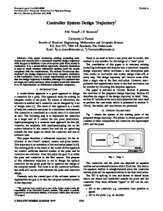
There is no need to have a real plant and its model, this method is also suitable for the design of a “new” plant. The contribution of this paper is to structure existing modelling techniques and theories into a systematic stepwise design trajectory which facilitates a less error-prone path from model to realization and makes design trade-offs at every step. The design trajectory will involve more effort than a single step to the final realization. However, unexplainable and unpredictable faults in the final realization can be avoided by following this stepwise approach. The paper is outlined as follows: Section II presents the overview of the proposed design trajectory. Section III describes the stages of the design trajectory in detail. Then, section IV introduces the tools and equipment that were used to perform the case study which is presented in section V. Finally, discussion and conclusions are presented. II. D ESIGN T RAJECTORY Fig. 1 shows the system at the starting point of the proposed design trajectory. The system is chosen generic and consists of three components: the controller, the input/output (I/O) and the plant.
Controller
O
I
I O
Plant
Model Simulation PC Fig. 1.
Stage 0
The controller and the plant are depicted as separate entities and are denoted in boxes with a filled line. The choice for separate entities is straightforward since the controller and the plant will be separated entities in the final realization. The I/O is split-up in two and shown in dotted boxes which are drawn half-inside/half-outside the plant and the controller. Now three different “types” of I/O can be concerned: • I/O in the controller, e.g. conversion from position to speed. • I/O in the plant, e.g. an encoder.
1910
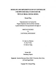
I/O outside the plant and controller, e.g. an encoder interface. This explicit structure ensures a consistent view for the I/O through the whole design trajectory and makes the design less error-prone. The arrows between the I/O boxes denote the interconnection, which in the final realization stage are the cables. The three components (controller, plant and I/O) are surrounded by a dotted box which is the realization “form” of the components. The realization form can be model, code or real. The outer solid box is the platform on which the model or code is simulated/executed. In case the realization form is real there is no platform, e.g. this is the case with the final plant realization. In this case the figure shows that the controller and plant are simulated in the same modelling environment and are simulated on a so-called simulation PC. The proposed design trajectory discussed in this paper will deal with a system that is build from one controller and one plant. Future research is necessary to extend to distributed controllers or hierarchical controller structures. However, the plant is always considered as one plant even if it consists of many individual components for example, multiple motors and multiple encoders. The reason for this is to keep the simulation process straightforward. Otherwise, a distributed plant simulation is necessary, which is not trivial. In case the plant is too computational intensive, distributed plant simulation cannot be avoided. Fig. 2 shows the proposed six “stage” design trajectory. A stage is a point in the design trajectory to test/experiment for a set of specific goals. The design trajectory presented here shows the basic case of a single controller with a single plant. Some stages will seem unnecessary/trivial but will become useful for more complex cases where multiple controllers and/or safety layers come into play. In the basic case of one controller, a transformation to stage 4 with a real plant or stage 6 is possible for which many tools are available [11], [12] and [14]. However, the emphasis in this paper is on the stepwise refinement from stage 1 to stage 6. The stages are numbered from one to six instead of named. The numbering is to avoid naming issues among terms commonly used for the described techniques. Table I shows names which could be applied to certain stages. •
Series 2 Simulation Co-Simulation Co-Simulation ... ... Realization Rapid Prototyping
TABLE I C OMMON N AMING C ONVENTIONS
The xIL terms are mentioned in [6], they mean Model, Software, Processor or Hardware In the Loop. The flow is from stage 1 to stage 6 (See Fig. 2). All stage transformations (automatic code-generation) are performed
I
I O
Plant
Model Simulation PC
2
Controller
O
I
I O
Code
3
Model Simulation PC
Controller
O
I
I O
Code Simulation PC
4
Plant
Plant
Model Simulation PC
Controller
O
I
I O
Plant
Code Test + RTOS
5
Model RT−Sim
Controller
O
I
I O
Plant
Code Target + RTOS
6
Controller
Model RT−Sim
O
I
Real−Time
Series 1 MIL SIL PIL HIL HIL ... ...
O
Simulated Time
Stage 1 2 3 4 5 6 ...
1
Controller
I O
Real Plant
Code Target + RTOS
Fig. 2.
Design Trajectory
from stage 1 to the corresponding stage. The design trajectory is roughly split-up in two parts, the simulated-time part and the real-time part. The real-time plant simulation dictates a fixed step-size integration method, since multi-step/variable step-size methods are not computationally bounded. In order to make a good comparison between the stages a fixed step-size integration method will be used for the simulated-time part. For the same reason a choice must be made for the interaction between the controller and the plant. Basically there are two interaction schemes [1]: • Steer as soon as possible (variable delay). • Steer with one sample delay (constant delay).
1911
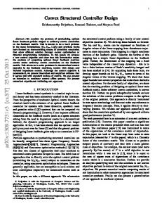
The delay is a computational delay, caused by using a computer to implement the control law. Both interaction schemes can be chosen, the design trajectory allows both. The choice is made for the “one sample” delay approach because it can be easily modelled by a unit delay. In case of a variable delay the computational delay has to be estimated, which is difficult or not possible since the target platform (realization) may still be unknown. Besides timedriven (synchronous) control there is event-driven (asynchronous)control [2], [7]. The proposed design trajectory allows both approaches but the latter is not discussed. Fig. 3 depicts the interaction between the controller and plant for stages 1,2 and 3. It shows how the simulation time (continuous and discrete) and the computational time relate. Note that there is synchronization between the plant (continuous-time) and the controller (discrete-time). The unit delay can be observed from the dotted arrow pointing from ‘td ’ to ‘tc+10 ’. td
td+1
td+2
tc
tc+10
tc+20
Computation time
Simulation−Time Discrete−Time Controller
Computation time
Simulation−Time Continuous−Time Plant
Fig. 3.
Simulated-Time relations
Fig. 4 depicts the interaction between the controller and plant for stages 4 and 5. Note that the continuous and discrete time are no longer synchronized (‘td ’ connects in this case to ‘tc + 11’). Furthermore the computation of a step must be finished before the next. Whereas in the simulation the next step will “wait” until the previous step has finished. td
td+1
td+2
Computation time
Real−Time Discrete−Time Controller tc+11
Computation time
Real−Time Continuous−Time Plant
tc
Fig. 4.
tc+10
Real-Time relations
tc+20
An error will be introduced by the asynchronous interaction. This could be solved by extending the I/O in these stages, however since the final realization will not have this “extended” I/O, it is not done. The real plant reacts infinitely fast and will be time-synchronous. III. S TAGES The design trajectory will be explained per stage. Note that the Real-Time simulation system (“RT-Sim” in Fig. 2) for the plant simulation can be any PC that is fast enough for (real-time) simulation. The Test system on the controller side (“Test” in Fig. 2) can be any commercial off-the-shelf (COTS) platform for the purpose of helping on deciding the final target platform. A. Stage 1 In this stage both the controller and plant are simulated in the same modelling environment/tool on the same Simulation PC. The plant model will be simulated in continuous time to approximate the continuous behavior. Although in general, sophisticated variable step-size numerical integration methods are most effective, a fixed step-size numerical integration method is used in this stage. This is to ensure that the computation time of the plant simulation is bounded, which is necessary in stages 4 and 5 to perform real-time plant simulation. The step-size of the numerical integration method has to be chosen to adequately handle the plant dynamics [3]. However, the step-size must be chosen such that real-time simulation of the plant model is possible. The simulation will be used to analyze the plant behavior and optimize the controller. Furthermore, the I/O needs to be considered here. This stage can be called Model-In-the-Loop Simulation. B. Stage 2 In this stage the controller runs outside the simulation as an executable. The I/O that is half-outside the controller runs in the simulation along with the plant model. In order to run the controller as an executable, code is generated from the controller model and compiled into an executable. The controller runs simultaneously with the model simulation of the plant. The verification test is obvious: the simulation results here should be identical to the simulation results of stage 1. In principle, no discrepancies are expected, because the control-laws executed in simulation and executed in the generated code behave identical: the same code runs on the same type of processors. The purpose of this stage is to perform a quick check that code can be generated from the model and functionally yields exactly the same results as the simulation in stage 1. Basically, this is a check if the code generator from the modelling tool works as expected. Furthermore, this is a check if the I/O is correctly dealt with. This stage can be skipped if there is enough confidence in the automatic code generation capabilities of the tool and correct dealing with the I/O.
1912
C. Stage 3 In this stage the controller runs on a separate Simulation PC. The I/O that is half-outside the controller is incorporated on the Simulation PC. The controller runs in a non-real-time environment but as a single task on a separate computer. The controller runs simultaneously with the model simulation of the plant. As in stage 2, the verification test is obvious. This stage is used to obtain a rudimentary estimation of the CPU usage. This stage is more useful when a larger part of the software than only the controller software needs to be tested. D. Stage 4 In this stage both the plant and controller run in realtime on two separate Computers: the Test System for the controller and the Simulation PC for the plant (note that this Simulation PC now runs a real-time operating system). The I/O that is half-outside the controller runs on the controller-side. The I/O that is half-outside the plant runs on the plant-side. Because in stage 1, a fixed step-size numerical integration method was chosen, both pieces of code generated from the model (controller and plant) are functionally identical to stage 1. Although, only the runtime environment is different, the effect on the simulation results is considerable. The communication between the plant and controller is no longer synchronized as was the case in the previous stages. To ensure accurate values for the plant on moments of sampling the plant is simulated at a higher frequency than the controller. e.g. the controller at 1 kHz, the plant at 10 kHz. Although the final target system is not used for the controller, this stage can be considered as Hardwarein-the-loop-Simulation since various COTS Test Systems can be used to determine the final Target System. By choosing a Test System similar to previous stages, only the migration of the nature of time is considered here. The constraints posed by the Target System are dealt with in the next stage. The verification step is not obvious: due to the realtime setting, no synchronized communication between the plant and controller and limited computation time, simulation results differ compared to those in the previous stages. In this stage the real-time behavior of the controller can be studied and accurate processor and memory usage can be determined in order to determine the target system and the target I/O. Trade-offs can be made in this stage, e.g. selecting a fast target system or a less computational intensive controller. E. Stage 5 In this stage the Target System replaces the Test System at the controller side. (The target system is the system that will be used in the end product.) Basically the transformation to stage 4 is the same as this stage. However, the transformation to this stage may be complicated by specific compilers and/or hardware resource limitations. Hence, the transformation to this stage will take more time and should be taken after the hard real-time behavior is analysed in the previous stage. The verification test should show similar behavior compared to the previous stage. Similar but not identical since
the timing of the target system may differ from the Test System. If the verification test is successful the real plant can be connected. F. Stage 6, the final stage In this final stage, the plant model is replaced by the real plant. Due to the consistent treatment of the I/O only the cables-ends of the (plant) Simulation System need to be connected to the real plant. The controller and the Target System are the same as in the previous stage. Differences in the verification test compared to those in the previous stage are caused by the difference between the plant simulation and the real plant. Hence, this is more a test on the quality of the plant model than on the controller and target system. However, since this is the end system the behavior of the system should satisfy the requirements. IV. T OOLS AND E QUIPMENT Before explaining the design trajectory on a case study, first the tools and equipment are introduced. A. Simulation and code generation tool 20- SIM 20- SIM [9] is a CACSD tool for modeling and simulation of plant dynamics, design and testing of control laws. Furthermore, it has a template-based code generation facility. This means that the code needed in the various stages is generated by 20- SIM, whereby the target-specific code is written in the template. The code generation functionality of 20- SIM thus combines the submodels from which code needs to be generated with the framework / device driver code as specified in the template. The coupling with I/O hardware is kept outside the models to keep the model itself clean from code generation and target-specific issues. This is to guarantee that the stages of the design trajectory are as independent as possible. This part is covered in CCE, the Command and Control Environment, which also features on-target testing with real-time data logging. B. I/O interconnection In stage 4 and 5, communication between the controller and plant is between two computers, whereas the I/O signals are the real I/O signals flowing between the Controller and Plant. The plant reads in the real signals (e.g. a PWM signal) from the controller and generates real sensor signals (e.g. an encoder quadrature signal). We have chosen to use a Field Programmable Gate Array (FPGA) that performs the signal processing [8]. Although for the steering signal generation and measurement signal acquisition standard interface devices (PWM generator resp. encoder) can be used, in this set up the FPGA is also used on the controller. This results in a symmetric setup, which is more straightforward to maintain. Furthermore, this gives more flexibility, and possibilities to choose where certain processing activities should be placed (a kind of Hardware / Software Codesign).
1913
C. plant The basic plant used for the case presented here, consists of a Maxon RE25 20 Watt DC motor, that drives a rotational load via a stiff belt, a so-called “Pinch”. A pinch is a component of a paperpath of a copier, which transports a sheet of paper. In the paperpath multiple pinches are cascaded to transport sheets of paper. For now we consider a single pinch driven by one motor. The 500 slit rotary encoder is mounted on the motor axis, because that gives a better controller performance [5]. The signal is acquired with quadrature demodulation, resulting in a resolution of 2000 pulses/revolution. The motor is controlled by applying a certain voltage through an H-bridge amplifier. The H-bridge used operates at 22 Volts and is limited to a maximum current of 1 Ampere.
Fig. 5.
System Overview
- measured), so that the velocity of the profile must be integrated. Furthermore, the encoder delivers an amount of pulses, which is divided by 2000 to obtain the measured angular position (in revolutions). The controller output is the dutycycle ([-1,1]) for the PWM.
D. Target and Test Systems These systems consists of a PC104+ CPU board with a 600 MHz x86 compatible CPU, supplied with 256 MB RAM and a 32 MB Flash disk which contains the Debian Linux operating system with the RTAI [13] real-time extension. An FPGA board is connected to the CPU board via the PCI bus in order to perform the I/O operations. In this setup the configuration for the FPGA contains a pulse width modulated output and encoder quadrature input. The PWM output signal has a frequency of 16kHz, the duty cycle can be set in 2048 steps and has a separate directional signal output. The CPU sets the duty-cycle and direction and the FPGA keeps these values until a new value has been received. The encoder input increments a counter at the FPGA on every pulse received from the encoder (the index pulse will not reset this counter). The CPU can read this counter.
Fig. 6.
PID Controller
The plant (Fig. 7) is modelled using iconic diagrams representing the differential equations that describe the dynamic behavior. The input of the plant is the PWM dutycycle ([1,1]), which is amplified using the H-bridge. The output of the plant is the motor velocity [rev/s], which is transformed to an encoder quadrature signal by the I/O. The plant is simulated with a step-size of 0.0001 s (10kHz).
E. Simulation PC and Real-Time Simulation System The Simulation PC is a cots 2.4 GHz x86 compatible CPU, supplied with 512 MB RAM which runs windows XP. For the real-time simulation, the system runs the Debian Linux operating system with the RTAI [13] real-time extension. V. C ASE S TUDY, DESIGN TRAJECTORY APPLIED
Fig. 7.
The ideas presented in this paper were tested on the basic plant described in the previous section.
Plant Model
B. Results
A. Case description The overview of the system is shown in Fig. 5. From the controller and plant submodels code was generated. The I/O was: • simulated in stages 1,2 and 3. • emulated by the FPGA in stages 4. • real on the plant side in stage 6. The Test system in Stage 4 and the Target system of Stage 5 were identical, thus, stage 4 and stage 5 are the same for this case. For the controller a basic PID controller is chosen, as depicted in Fig. 6, operating at 1 kHz. The control goal for this case is to follow the velocity profile. However, the controller input is the error in the angular position (desired
This section summarizes the results. Fig. 8 shows a controller and plant simulation (stage 1). It serves as result to compare to for the rest of the stages. The velocity signal has small spikes, which are caused by the calculation of the discrete-time derivative of the angular position: the velocity signal is calculated by subtracting two consecutive angular position sample divided by the sample time. In this case, the resolution of the velocity is 0.5 [rev/s]. For this reason the comparison between the stages is made based on the encoder pulses instead of the velocity. Fig. 9 shows the error in encoder pulses of stages 2 to 6 compared to stage 1. The amount of encoder pulses in these stages were subtracted from the amount of encoder pulses of stage 1.
1914
VI. D ISCUSSION AND C ONCLUSION
Fig. 8.
A refinement trajectory for the design of a plant and its control has been proposed. A basic case study shows that trajectory was successfully gone through with the given tools and equipment. However, the case itself is too limited to show the benefits of all the stages in the design trajectory. As future work, we plan to apply the design trajectory on the Boderc [10] set up which is more complex, namely a distributed control computer system consisting of 4 PC104+ nodes which controls a paperpath system driven by 5 DC motors. Obviously, the design trajectory will be extended to also cover distributed embedded computing nodes. A fixed step-size integration was used to ensure real-time behavior. A very basic approach; generate an exception when the real-time behavior is violated could be used to allow different integration methods. In this case when the simulation PC is fast enough the simulation can be performed.
Stage 1: Simulation Results
R EFERENCES
Fig. 9.
•
•
•
Simulation of stages 2 to 6, difference in encoder pulses
Stage 2 and 3 show identical results with the simulation of stage 1. Measurements of processor usage in these stages show that the execution time for one cycle of the controller was about 0.55 μs. A crude estimation for the target system based on the difference of processor frequency is 2.2 μs. This is much smaller than 1 ms, hence no real-time performance issues are expected. Stage 4 shows similar results but the position error is one encoder pulse, which is caused by the fact that the simulation does not run synchronized (Fig. 4). In this stage experiments were performed with the Test System and the Target System. The processor usage for the controller including the I/O communication in this stage was about 4.1 μs for the Target System. This shows it will be a suitable final Target System. However, it is overdimensioned for this simple case. Stage 6 shows that the behavior differs from the simulation. This is caused by the fact that the model is not identical with the real plant (e.g. a plant property which was not taken into account in the plant model or a parameter which is not precise).
˚ [1] Astrom, Karl J., Wittenmark Bj¨orn, Computer Controller Systems : Theory and Design, Prentice Hall, ISBN 0-13-314899-8, 3rd ed, pp. 328-330, 1997. ˚ en, Karl-Erik, A simple event-based PID controller. In: Preprints [2] Arz´ 14th World Congress of IFAC. Beijing, P.R. China, 1999. [3] P.P.J. Bosch, van den, and A.C. Klauw, van der, Modeling, Identification and Simulation of Dynamical Systems CRC Press Inc., ISBN 0-8493-9181-4, 1994, pp. 195. [4] J. F. Broenink and G. H. Hilderink, A structured approach to embedded control systems implementation, In M. W. Spong, D. Repperger, and J. M. I. Zannatha, Eds., 2001 IEEE International Conference on Control Applications. Mexico City, Mexico, 2001. [5] Coelingh, H.J., Design support for motion control systems, University of Twente, PhD thesis, ISBN 90-36514118, 2000. [6] R. Isermann, J. Schaffnit, and S. Sinsel, Hardware-in-the-loop simulation for the design and testing of engine control systems, Control Engineering Practice, vol. 7, pp. 643-653, 1998. [7] Sandee, J.H., W.P.M.H. Heemels and P.P.J. v.d. Bosch, Event-driven control as an opportunity in the multidisciplinary development of embedded controllers, Proceedings of the American Control Conference, Portland, Oregon, USA, pp. 1776–1781, 2005. [8] Visser, P.M., M.A. Groothuis and J.F. Broenink, ”FPGAs as versatile configurable I/O devices in Hardware-in-the-Loop Simulation”, in: Work in Progress at the 25th IEEE International Real-Time Systems Symposium , in: The 25th IEEE International Real-Time Systems Symposium, Lisbon, Portugal, 5-12 - 8-12-2004, pp. 41-44, 2004. [9] 20-Sim, modelling and simulation package, Controllab Products Inc., Enschede, The Netherlands, [online] http://www.20sim.com, 2006. [10] Embedded Systems Institute, ”Boderc Project”, [online] http://www.esi.nl/site/frames.html?/site/news/history/2002/boderc.html, 2002. [11] dSpace prototyping systems, dSPACE Inc., Novi, USA, [online] http://www.dspaceinc.com/, 2006. [12] LabVIEW REAL-TIME, National Instruments Corporation, Austin, USA, [online] http://www.ni.com/realtime/control design.htm, 2006. [13] RTAI : the RealTime Application Interface for Linux, [online] https://www.rtai.org/, 2006. [14] xPC Target 3, The Mathworks, Massachusetts, USA, [online] http://www.mathworks.com/products/xpctarget/, 2006.
1915