camera and a 3D LIDAR sensor, separately and in combination. Early and ... vehicles. Convolutional Neural Networks (CNN) is used in this work as classifier in distinct situations: having a single sensor ... used sensor in pedestrian classification and detection [5]. ... âfully occludeâ, âunknowâ and âdon't careâ region objects,.
Multimodal CNN Pedestrian Classification: a Study on Combining LIDAR and Camera Data Gledson Melotti1 , Cristiano Premebida1 , Nuno M. M. da S. Gonc¸alves1 , Urbano J. C. Nunes1 and Diego R. Faria2 Abstract— This paper presents a study on pedestrian classification based on deep learning using data from a monocular camera and a 3D LIDAR sensor, separately and in combination. Early and late multi-modal sensor fusion approaches are revisited and compared in terms of classification performance. The problem of pedestrian classification finds applications in advanced driver assistance system (ADAS) and autonomous driving, and it has regained particular attention recently because, among other reasons, safety involving self-driving vehicles. Convolutional Neural Networks (CNN) is used in this work as classifier in distinct situations: having a single sensor data as input, and by combining data from both sensors in the CNN input layer. Range (distance) and intensity (reflectance) data from LIDAR are considered as separate channels, where data from the LIDAR sensor is feed to the CNN in the form of dense maps, as the result of sensor coordinate transformation and spatial filtering; this allows a direct implementation of the same CNN-based approach on both sensors data. In terms of late-fusion, the outputs from individual CNNs are combined by means of learning and non-learning approaches. Pedestrian classification is evaluated on a ‘binary classification’ dataset created from the KITTI Vision Benchmark Suite, and results are shown for each sensor-modality individually, and for the fusion strategies.
I. INTRODUCTION Despite of the numerous traffic signals, crosswalks and pedestrian safety signage, the number of accidents between cars and pedestrians is sadly very high. Thus, the development of advanced perception systems (e.g., pedestrian detection) is a promising step forward to reduce drastically the number of accidents on the roads. Therefore, sensor-based pedestrian detection systems have attracted many studies from the scientific community [1], [2], [3], [4]. The recent advances in pedestrian safety systems are remarkable, but it is still a challenging task because, among other reasons, light influence and appearance (scale, texture, position) of pedestrian is subject to numerous changes and also occlusion [3]. An important item in a pedestrian classification system is the type of sensor used to capture road scenes. In this regard, one can categorize the sensors as passive or active. Cameras, which belong to the first category, are the most widely used sensor in pedestrian classification and detection [5]. However, passive sensors have disadvantages as illumination 1 The authors are with the Dept. of Electrical and Computer Engineering, Institute of Systems and Robotics, University of Coimbra. {gledson.melotti,cpremebida,nunogon,urbano}
@isr.uc.pt. 2 Diego Resende Faria is with the School of Engineering & Applied Science Aston University, UK. {d.faria}@aston.ac.uk.
variations effects and night vision difficultness [6]. On the other hand, active sensors, like automotive radar and LIDAR [6], [7], [8], are more robust against illumination changes and also have the pro of measuring the range/distance directly. The cons of the LIDAR sensors are the high prices and the moving parts (however, some recently launched solid-states LIDAR do not use moving mechanisms). There are several datasets on pedestrian classification, a review can be find in [5], such as: INRIA, NICTA, Caltech, Daimler Monocular, Daimler Multi-Cue, ETH and KITTI. In this paper we will use a ‘classification’ dataset built from the KITTI suite [7]. KITTI is a state-of-the-art benchmark for pedestrian detection in urban and road environments and has the key advantage of providing synchronized and calibrated data from monocular cameras and a 3D-LIDAR. Furthermore, it provides examples of “partly occluded”, “fully occlude”, “unknow” and “don’t care” region objects, which make the classification or detection problem more challenging and realistic. In this paper, we present a study on pedestrian classification using deep convolutional neural network (CNN) based on the TensorFlow architecture. CNN-based pedestrian classification is performed on color images (RGB channels) from a monocular camera and also on 3D LIDAR data (depth and reflectance’s intensity level), in combination and separately. LIDAR point clouds are used to generate highresolution (dense) depth and reflectance maps through a bilateral filter (BF) implementation. Although some papers address pedestrian detection1 and classification/recognition interchangeably, the concept of classification and detection are not the same. In short, and ignoring the time variable dependency, the former depends essentially on a classifier and correlate feature-space, while the later has to deal with unknowns in position and size/scale and depends on many factors related, but not limited, to: hypothesis generation (e.g., clustering, salient region generation), hypothesis confirmation (a classifier), post-processing (e.g., non-maximum suppression). However, in this work the classification problem is particularly addressed motivated by the fact that we are interested in exploring the contribution of monocular-camera and LIDAR data without influence of further elements. Thus, the contributions of this work are: (i) study the capacity of deep-learning on LIDAR-based maps, considering the range and reflectance data, applied to pedestrian classification; (ii) evaluation of the classification 1 The
same rationale applies to ‘cyclist’ or ‘cars’ categories.
4 3 2 1
performance of early and late fusion strategies, based on learning and deterministic fusion techniques. The structure of this paper is as follows: in Section II related works are revisited. LIDAR based depth and reflectance maps are explained in Section III. Section IV describes the dataset, and the classification approaches are presented in Section V. Results and conclusions are provided in Sections VII and VIII respectively. Z
0
-1 -2 -3
25
X
20
15
10
II. RELATED WORK
Fig. 1. Example of a point-cloud from the HDL-64E Velodyne 3D LIDAR (extracted from KITTI dataset). In the scene, it is possible to see a pedestrian.
5 15
Pedestrian classification/recognition is a key research and technological topic in the automotive industry and academia, since it is the baseline of advanced pedestrian detection systems for ADS, ADAS, and automotive protection systems. In [4], an experimental study on pedestrian classification is conducted, exploring several combination of classifiers (SVM, feedforward neural networks and K-nearest neighbors) and presents a comparative analysis of global, local, adaptive and nonadaptive features (PCA, Haar wavelets and local receptive fields). The authors investigated the relationship between classification performance and training sample size. Finally, they concluded that global features performance is lower than local ones, and that adaptive features are better than non-adaptive. In a more recent study [5], pedestrian classification is carried out using multi-domain (visible and far-infrared (FIR)) and multi-modality data (intensity, depth and motion). The main contributions in [5] are a public dataset with far-infrared and visible images, and a study on features extracted from both camera spectra. In this regard, intensity self-similarity (ISS), local binary patterns (LBP), local gradient patterns (LGP) and histogram of oriented gradients (HOG) were used for feature extraction. The study was performed considering individual methods and a fusion approach. For pedestrian classification the FIR method has shown better results than the other methods. In the study developed in [9] it is possible to verify the importance of considering a four-component combination for pedestrian detection. These components are feature extraction, deformation handling, occlusion handling, and classification. Then the learning formulation maximizes their strengths through a cooperative process, that improves pedestrian detection accuracy. Existing methods and approaches on pedestrian classification (and object detection in general) use, most commonly, camera-based solutions [10]. However, more recently the number of works using LIDAR are rising in prominence [11], [12], [13], [14], [15], [16]. In this paper, we explore the multimodality fusion by combining distinct sensors modalities (camera and LIDAR) and, additionally, by combining different data from the same sensor modality (i.e., range and reflectance from a LIDAR). Furthermore, we investigate two schemes for fusion (early and late) where in the late fusion we study numerous approaches.
5
10
0
-5
Y
III. DEPTH AND REFLECTANCE MAPS FROM LIDAR DATA The motivation is to use 3D point cloud to contribute to the pedestrians classification using a deep CNN. For instance, Fig. 1 shows a 3D point-cloud, gathered by a HDL-64E Velodyne LIDAR, having a pedestrian in the scene. Let consider the LIDAR output (or scan) in the form of a point-cloud, defined as a set of points in 3D Cartesian coordinate system (P3R ), where the variables of interest are the range (distance) and also the reflectance (intensity). The set of points P, from a LIDAR scan, is assumed to be in the image-plane reference system; i.e., P is in pixel coordinates and is the result of a coordinate transformation from R3 to the camera coordinate system and then to the image-plane. P contains the points {p1 , p2 , . . . , pn } and each pi = (u, v, ra, re)i represents the position in pixel coordinates (u, v)i , the range/distance value rai , and rei is the reflectance as measured by the LIDAR. Therefore, to get the depth map (DM) and a reflectance map (RM) it is necessary to estimate the values of rai and rei in unsampled locations of the LIDAR’s projected pixel-plane (hereafter, it is called a Map). One way to get a DM and/or a RM is by means of spatial filtering techniques, from image processing area, which can be implemented by a sliding-window (a mask) technique in a given space domain. Spatial filters, in image processing, act directly on the pixels domain by combining the ‘intensity’ of a group of pixels (belonging to the window) to estimate the desired ‘intensity’ value of the central-pixel of the mask [17]. In other words, and assuming a mask M with size m × n, the ‘intensity’ value to be estimated/predicted is, in this work, the variables rai and rei from the LIDAR points P. In this work, we decided to apply the bilateral filter, which takes into account the distance and intensity of the pixels and the formulation of the BF can be expressed as follows [17]: r0∗ =
1 W
∑
Gσs (||x0 − xi ||)GσR (|r0 − ri |ri
(1)
xi ∈M
where x0 = (u, v)0 is the location of interest, which is the center of M, and r0∗ is the variable to be estimate, i.e., the range and reflectance (ra; re) at x0 . W is a normalization factor that ensures weights sum to one, Gσs is inversely proportional to the Euclidean distance between the center of M and the sampled locations xi , and GσR controls the
TABLE I S UMMARY OF THE CLASSIFICATION DATASET Training set Validation set Testing set
n# positives = 2827 n# negatives = 29849 n# positives = 314 n# negatives = 3316 n# positives = 1346 n# negatives = 14213
Fig. 2. This picture illustrates, considering a given image-frame (1st row) from KITTI dataset, a LIDAR scan as projected to the image-plane (the 2nd row), and the corresponding DM and RM maps respectively.
influence of the sampled points based on their values ra or re, depending on the case. If r0 does not exist in M, it was considered the value r0 = min(ri ), ∀ri ∈ M. An example of range (DM) and reflectance (RM) maps, by using bilateral filtering on a projected 3D LIDAR’s point-cloud, is shown in Figure 2. Notice that both maps, DM and RM, use only data from the LIDAR and therefore camera data is considered for calibration and visualization purposes. IV. DATASET We composed a “classification” dataset from the 2D object-detection dataset of KITTI, where the classes are given in the form of 2D bounding box tracklets: Car, Van, Truck, Pedestrian, Person (sitting), Cyclist, Tram and Misc. In this paper the classes were separated in two classes/categories of interest: pedestrian and non-pedestrian i.e., a binary classification problem. The number of pedestrian examples comprises 4487 cropped-images , while the non-pedestrian class has 47378 cropped-images 2 . Table I gives a summary of the binary classification dataset employed in this study. Figure 3 shows some pedestrian (positives) and nonpedestrian (negatives) classification examples for the sensor modalities used in this work i.e., camera and LIDAR. For the LIDAR, Fig. 3 shows depth and reflectance maps. 2 It was considered 70% for the training set (10% of that for validation) and the remaining 30% for the testing set.
Fig. 3. In the first row we have examples of pedestrians and non-pedestrians from the monocular camera. The last two rows show the corresponding depth and reflectance maps generated from LIDAR data.
V. CLASSIFICATION USING CNN Knowing that deep CNN attained good performance, AlexNet architecture was chosen to perform pedestrian classification3 [18]. The classifiers were trained using the Keras and TensorFlow packages [19]. VI. SENSOR FUSION STRATEGIES The combination, or fusion, of data from distinct sensors, in the scope of object recognition, is usually performed by early fusion or late fusion schemes [20]. In this work, we considered both information fusion strategies. In the sequel, we describe the way both strategies were used to combine data from camera and LIDAR for pedestrian classification. 3 We use batch normalization in the first two layers of the AlexNet CNN. In the last layer a softmax activation function with two classes and dropout of 50% was used. All images were re-sized to the size of 227 × 227. The network was trained on 30 epochs, batch size equal 64, stochastic gradient descent optimizer with lr = 0.001 (learning rate), decay = 10−6 (learning rate decay over each update), momentum = 0.9, and categorical cross entropy as loss function.
A. EARLY FUSION For this case, we trained a CNN with 3 channels where each channel received data from one modality, as follows: the first channel of the input layer received gray-scale images (from the camera), the second and third received the depth and reflectance maps (from LIDAR) respectively. It is an efficient and simple strategy to implement, and the classification performance is higher than a single-modality CNN model as demonstrated by the results (in Sect. VII). B. LATE FUSION The number of methods able to combine classifiers outputs is extensive. On one hand, there are many simple (nonlearning) rules one can use, such as: average, maximum, minimum, product, and so on. On the other hand, there are learning-based techniques which usually achieve superior performance in classification but require more complex implementations; these techniques depend, essentially, on a model (generative or discriminative) learned from the training set. In this study, we will provide results using some simple rules, namely: average, minimum, maximum, and normalized-product (which can be understood as a Naive Bayes rule). Also, two more advanced fusion approaches were implemented: one using Jensen-Shannon divergence, and another employs a linear-SVM to combine the CNNclassifiers. 1) NON-LEARNING FUSION TECHNIQUES: Denoting Li the confidence (or probability) score yielded by deepmodels CNNi , (i = 1, · · · , nc), where nc = 3, CNN1 is the camera-based model, CNN2 comes from DM (depth), and CNN3 refers to RM (reflectance) model. Four ‘simple’ fusion rules are considered: average FMean , maximum FMax , minimum FMin , and Naive-product FProd . The average rule simply calculate the simple mean of the CNN-classifiers outputs 1 nc FMean = nc ∑i=1 Li . The maximum rule outputs the maximum value over the classifier responses, FMax = maxi {Li }, while the minimum rule is FMin = mini {Li }. Assuming classifiers’ independence given the sensors modalities, the Naive-product rule is expressed by FProd =
∏nc i=1 Li nc ∏i=1 Li + ∏nc i=1 (1 − Li )
(2)
To avoid non-informative likelihoods i.e., close-to-zero values due to the product operation, a small additive-smoothing Prior was added to Li . 2) JS BASED STRATEGY: This fusion strategy resorts to weights based on Jensen-Shannon (JS) divergence computed from the training set. The fusion approach is a probabilistic mixture model using the current test set posterior given by a specific classifier and the weights assigned to each modality as follows: N
P(γ|λ1 , λ2 , ...λn ) = α × ∑ P(λi |γ) × wi ,
(3)
i
where P(γ|λ1 , λ2 , ...λn ) is the fusion posterior; {P(λ1 |γ), P(λ2 |γ), ...P(λn |γ)} are probabilities attained
using CNN for each sensor modality; wi is a JS-weight for each modality learned from the training set observations; and α is a normalization factor (taking into account all classes). The Kullback-Leibler (KL) divergence [21] is an asymmetric measure of the difference between two probability distributions. However, a symmetric measure is obtained by averaging the KL divergence, also known as JensenShannon divergence (a.k.a. total divergence to the average [22]). Based on that, the divergence between prior and posterior distributions is computed, where the prior is the global weight learnt given the training set (see [23]) and the posteriors in this model are given by the classified frames precedent to the current frame from the training set. The weights for each modality are calculated as follows: {1:t−1}
DKLi (P(oi
) k P(wgi )) =
t−1 l=1
{1:t−1}
DKLi (P(wgi ) k P(oi
t−1
)) =
P(ol )
∑ P(oli ) P(wig ) , P(wg )
∑ P(wgi ) P(oli ) ,
l=1
(4)
i
(5)
i
� � �� DJSi = 0.5 × DKLi P(oi ) k P(wgi ) + DKLi P(wgi ) k P(oi ) , (6) wi =
DJSi , ∑i DJSi
(7)
where wi is the resulting updated weight for current fusion, P(wgi ) = wgi represents the global weight learnt from the training set using a specific weighting strategy (e.g., entropy-based weighting, residual probability energy, etc., as described in [23]); P(oi ) = P(λi |γ), which is the previous classification probability {t − 1, ...,t − n}, i.e., posteriors corresponding to an ith modality; wi is weight based on JS divergence [23]. 3) SVM LATE FUSION APPROACH: In this case, a SVM classifier (working as a fusion-classifier) receives the outputs from the CNNs and then outputs a confidence score, or a decision, concerning the classification problem. Here, a SVM with linear-kernel (using the LibSVM library) was applied to operate as late fusion-classifier. The SVM is firstly trained by using the CNNs scores (Li from the training-set) and then, based on the trained model, the SVM is used on the testing-set to estimate the desired combined score. VII. EXPERIMENTS AND RESULTS All results, monocular camera (MC), depth map (DM), reflectance map (RM) and early sensor fusion (gray-scale image + DM + RM), were analyzed using F-score, recall and precision performance measures and ROC curves (area under the curve-AUC), allowing a more detailed and accurate analysis of the results, as showed in Table II. The F-scores, recalls and precisions were obtained considering a threshold of 0.5. The number of pedestrian and non-pedestrian examples is unbalanced, as shown in Table I, thus, F-score is here considered because it is a suitable performance measure for unbalanced cases.
TABLE II R ESULT OF CLASSIFIERS . C ALCULATIONS WERE MADE WITH A
F-score 0.8953 0.7886 0.8872 0.9053 0.9080 0.9082 0.8592 0.7931 0.9105 0.1794
0.5 TO OBTAIN THE F- SCORES VALUES .
Precision Recall Monocular Camera (MC) 0.8887 0.9019 Depth Map (DM) 0.8479 0.7370 Reflectance Map (RM) 0.8733 0.8811 CNN Fusion (Early) 0.9125 0.8982 Jensen-Shannon (JS) 0.9375 0.8804 Average (Mean) 0.9320 0.8856 Maximum (Max) 0.7695 0.9725 Minimum (Min) 0.9824 0.6649 Product (Prod) 0.9343 0.8878 SVM late fusion 0.4730 0.1107
0.9
0.9928 0.9769 0.9901
0.85
0.8 0.75
0.65
0.9966
0.6
0.9967
0
0.05
0.1
0.15
0.2
0.25
0.3
0.35
0.4
False Positive Rate
0.9963 Fig. 5. ROC curves, on the testing set, for the later sensor-fusion schemes: FMax , FMean , FMin , FProd .
0.9954 0.9969
Receiver Operating Characteristic-ROC
1
0.9023
JS; 0.9966 SVM;0.9023 Early fusion; 0.9966 JS*;[0.0056,0.8804] SVM*;[0.0117,0.1107] Early fusion*;[0.0082,0.8982]
0.95 0.9
0.8
0.85
True Positive Rate
0.9
0.85
0.7
0.9966
Camera; 0.9950 Depth; 0.9795 Reflectance; 0.9901 Camera*; [0.0107,0.9019] Depth*; [0.0125,0.7369] Reflectance*; [0.0121,0.8811]
0.95
True Positive Rate
AUC
Receiver Operating Characteristic-ROC
1
Max; 0.9963 Mean; 0.9967 Min; 0.9954 Prod; 0.9969 Max*; [0.0276,0.9725] Mean*; [0.0061,0.8856] Min*; [0.0011,0.6649] Prod*; [0.0059,0.8878]
0.95
True Positive Rate
THRESHOLD OF
Receiver Operating Characteristic-ROC
1
0.8 0.75 0.7 0.65
0.75 0.6 0.7 0.55 0.65 0.5 0.6
0
0.05
0.1
0.15
0.2
0.25
0.3
0.35
0.4
0.45
0.5
False Positive Rate
0.55 0.5 0
0.05
0.1
0.15
0.2
0.25
0.3
0.35
0.4
0.45
0.5
Fig. 6. ROC curves, on the testing set, for the early fusion using a CNN, and the curves for the late fusion suing SVM and JS divergence.
False Positive Rate
Fig. 4. Receiver Operating Characteristic (ROC) curves, on the testing set, for the sensors modalities evaluated.
Figure 4 shows the ROC curves, calculated on the testing set, for the CNN models using color-images (camera), depth maps (depth) and reflectance maps (reflectance). In addition, optimal operating points for threshold equal to 0.5 are shown in the curves and the values are indicated in the legend designated by the superscript (∗ ), followed by [FP, T P]. The curves are zoomed and displayed in the interval from 0 to 0.5, both for true positive rate (TP) and false positive rate (FP). Figures 5 and 6 show the ROC curves for the fusion strategies. The results for the deterministic fusion rules, obeying the late scheme as described in Sect. VI-B.1, are shown in Fig. 5, while the testing results for the early fusion (using a 3-channel CNN) and for the more sophisticated fusion strategies - using JS divergence and rescoring SVM are shown in Fig. 6.
Besides the ROC curves, the performance measures (sometimes called metrics) used in our evaluation allow us to compare, in a more accurate way, the following approaches: single modality CNNs (Table II and Fig. 4); non-learning late fusion (Fig. 5); early fusion using a CNN and the learningbased late fusions (Fig. 6). The area under curve (AUC) is, except for the late fusion using SVM, not enough for a fair comparison. Looking at the values of the optimal operating points and the F-score values (note that the reference threshold is 0.5 and the dataset is unbalanced), we can conclude the following: • For single modality, camera performs better than DM and RM. However, the classification performance using LIDAR reflectance (RM) is very promising; • Among the non-learning rules, the simple mean achieved good results. The maximum rule is very good in terms of TP but, the FP increases. The normalized product rule attained the best results among these fusion category;
For the learning fusion strategies, the linear-SVM had inferior performance. On the other hand, the JS (late) and the CNN (early) achieved equivalent performance. Finally, by comparing the single sensor modalities (camera or LIDAR) and the multi-modality fusion strategies, we can conclude that in all cases (except for the SVM rule) the combination of camera and LIDAR data increases the classification performance. Although such performance results were expected i.e., fusion vs single-modality is favorable to the former, it is to be noted the very promising performance due to the LIDAR’s reflectance maps. •
VIII. CONCLUSION AND REMARKS An approach for pedestrian classification based on deeplearning and data-fusion strategies, using camera and LIDAR data, has been presented in this paper. Pedestrians and nonpedestrians labels were extracted from the KITTI Object dataset. Therefore, we composed a ‘binary classification’ dataset consisting of pedestrian and non-pedestrian (all remaining categories). KITTI also provides the corresponding LIDAR scans, which contains the 3D coordinate points as well as the reflectance data. For the LIDAR data, and by using spatial filtering, we calculated depth (DM) and reflectance (RM) maps to allow a direct implementation of CNN-based models. Based on camera images and LIDAR maps, and using CNN as learning model, were considered two cases: 1) single-modality i.e., by training a CNN with image (camera), DM, and RM individually; 2) fusion schemes: early fusion, where a 3-channel CNN is trained using data from the three modalities; and late fusion, where non-learning (e.g., average, product, maximum) and learning techniques (JS divergence, SVM) were implemented and used to combine single-modalities CNNs. Experiments on both camera and LIDAR data were carried out to assess the classification performance of the single and multi-sensor modalities, early and late fusion schemes. From the experimental results reported in this paper, the fusion strategies attained the best results in comparison with the individual CNNs, as shown in the ROC curves and Table II. Finally, it is worth noting the promising results achieved by the LIDAR reflectance map approach. ACKNOWLEDGMENTS This work has been partially supported by “MATIS - Materiais e Tecnologias Industriais Sustent´aveis” (CENTRO-01-0145-FEDER000014), co-financed by the European Regional Development Fund (FEDER), through the “Programa Operacional Regional do Centro” (CENTRO2020) program; and partially supported by System Analytics Research Institute (SARI), Aston University, Birmingham, UK; and also by the Federal Institute of Esp´ırito Santo-Brazil.
R EFERENCES [1] T. E. Wu, C. C. Tsai, and J. I. Guo, “Lidar/camera sensor fusion technology for pedestrian detection,” in 2017 Asia-Pacific Signal and Information Processing Association Annual Summit and Conference (APSIPA ASC), Dec 2017, pp. 1675–1678.
[2] K. Li, X. Wang, Y. Xu, and J. Wang, “Density enhancement-based long-range pedestrian detection using 3-d range data,” IEEE Transactions on Intelligent Transportation Systems, vol. 17, no. 5, pp. 1368– 1380, May 2016. [3] S. Aly, “Partially occluded pedestrian classification using histogram of oriented gradients and local weighted linear kernel support vector machine,” IET Computer Vision, vol. 8, no. 6, pp. 620–628, 2014. [4] S. Munder and D. Gavrila, “An experimental study on pedestrian classification,” IEEE Transactions on Pattern Analysis & Machine Intelligence, vol. 28, no. 11, pp. 1863–1868, 2009. [5] A. Miron, A. Rogozan, S. Ainouz, A. Bensrhair, and A. Broggi, “An evaluation of the pedestrian classification in a multi-domain multimodality setup,” Sensors, vol. 15, no. 6, pp. 13 851–13 873, 2015. [6] A. Asvadi, L. Garrote, C. Premebida, and U. Nunes, “DepthCNN: Vehicle detection using 3d-lidar and convnet,” in Proc. of the IEEE 20th International Conference on Intelligent Transportation Systems (ITSC), Yokohama, Japan, 2017. [7] A. Geiger, P. Lenz, C. Stiller, and R. Urtasun, “Vision meets robotics: The kitti dataset,” International Journal of Robotics Research (IJRR), vol. 32, no. 11, pp. 1231–1237, 2013. [8] A. Asvadi, L. Garrote, C. Premebida, P. Peixoto, and U. J. Nunes, “Real-time deep convnet-based vehicle detection using 3d-lidar reflection intensity data,” in ROBOT 2017: Third Iberian Robotics Conference. Springer International Publishing, 2018, pp. 475–486. [9] W. Ouyang, H. Zhou, H. Li, Q. Li, J. Yan, and X. Wang, “Jointly learning deep features, deformable parts, occlusion and classification for pedestrian detection,” IEEE Transactions on Pattern Analysis and Machine Intelligence, pp. 1–1, 2018. [10] J. Zhu, S. Liao, Z. Lei, and S. Z. Li, “Multi-label convolutional neural network based pedestrian attribute classification,” Image and Vision Computing, vol. 58, pp. 224 – 229, 2017. [11] D. Matti, H. K. Ekenel, and J. Thiran, “Combining lidar space clustering and convolutional neural networks for pedestrian detection,” CoRR, vol. abs/1710.06160, 2017. [Online]. Available: http://arxiv.org/abs/1710.06160 [12] H. Wang, B. Wang, B. Liu, X. Meng, and G. Yang, “Pedestrian recognition and tracking using 3d lidar for autonomous vehicle,” Robotics and Autonomous Systems, vol. 88, pp. 71 – 78, 2017. [13] D. D. Pham and Y. S. Suh, “Pedestrian navigation using foot-mounted inertial sensor and lidar,” Sensors, vol. 16, no. 1, 2016. [14] J. Schlosser, C. K. Chow, and Z. Kira, “Fusing lidar and images for pedestrian detection using convolutional neural networks,” in 2016 IEEE International Conference on Robotics and Automation (ICRA), May 2016, pp. 2198–2205. [15] R. O. Chavez-Garcia and O. Aycard, “Multiple sensor fusion and classification for moving object detection and tracking,” IEEE Transactions on Intelligent Transportation Systems, vol. 17, no. 2, pp. 525– 534, Feb 2016. [16] T. Nagashima, T. Nagasaki, and H. Matsubara, “Object classification integrating estimation of each scan line with lidar,” in 2017 IEEE 6th Global Conference on Consumer Electronics (GCCE), Oct 2017, pp. 1–4. [17] A. McAndrew, A Computational Introduction to Digital Image Processing, 2nd ed. Chapman and Hall/CRC, 2015. [18] B. Zhou, A. Lapedriza, A. Khosla, A. Oliva, and A. Torralba, “Places: A 10 million image database for scene recognition,” IEEE Transactions on Pattern Analysis and Machine Intelligence, vol. 40, no. 6, pp. 1452–1464, June 2018. [19] F. Chollet et al., “Keras,” https://keras.io, 2015. [20] X. Chen, H. Ma, J. Wan, B. Li, and T. Xia, “Multi-view 3d object detection network for autonomous driving,” in IEEE CVPR, 2017. [21] S. Kullback, “Information theory and statistics,” J. Wiley & Sons, 1959. [22] I. Dagan, L. Lee, and F. Pereira, “Similarity-based methods for word sense disambiguation,” 35 Annual Meeting of the Assoc. for Comp. Linguistics and 8 Conf. of the European Chapter of the Assoc. for Comp.Linguistics: 56-63, 1998. [23] D. R. Faria, M. Vieira, F. C. Faria, and C. Premebida, “Affective facial expressions recognition for human-robot interaction,” in RO-MAN’17: IEEE International Symposium on Robot and Human Interactive Communication, Lisbon, Portugal, 2017.