However, the sudden availability of cheap 3D sensors such ... depth inputs on pedestrian detection using registered pairs .... Designating by J the spatial domain.
Pedestrian Detection Combining RGB and Dense LIDAR Data Cristiano Premebida, Jo˜ao Carreira, Jorge Batista and Urbano Nunes
Abstract— Why is pedestrian detection still very challenging in realistic scenes? How much would a successful solution to monocular depth inference aid pedestrian detection? In order to answer these questions we trained a state-of-theart deformable parts detector using different configurations of optical images and their associated 3D point clouds, in conjunction and independently, leveraging upon the recently released KITTI dataset. We propose novel strategies for depth upsampling and contextual fusion that together lead to detection performance which exceeds that of the RGB-only systems. Our results suggest depth cues as a very promising mid-level target for future pedestrian detection approaches.
I. I NTRODUCTION Reliable object/pedestrian detection is a key research goal in robotics and computer vision as it would greatly facilitate the practical deployment of autonomous robots. Pedestrian detection in images saw much progress over the last decade, which can be to a large degree owed to the success of the Histogram of Oriented Gradients (HOG) descriptor [1] and the sliding-window detection formulation. Recent benchmarks [2], [3], [4] have nevertheless demonstrated that there is much room for improvement when algorithms are tested on realistic scenes. Despite some promising attempts [5],[6], depth inference from a monocular optical camera is still an open problem. However, the sudden availability of cheap 3D sensors such as Kinect, has brought a renewal of interest in recognition approaches leveraging higher-level cues beyond image gradients, such as those readily available from range data. Kinect provides a dense depth map registered with an RGB image (RGB-D) on which standard detection machinery can be applied and this has stimulated much recent research in object detection [7],[8] articulated pose prediction [9] and scene understanding [10]. On the other hand, Kinect’s sensor is less reliable in outdoor scenes and has a maximum range of about 4 meters precluding pedestrian detection applications. By contrast, 3D laser range sensors, also known as laser scanner or Light Detection and Ranging (LIDAR), such as the Velodyne HDL-64E produce sparser point clouds, but can operate outdoors and have maximum ranges upwards of 50 m making them appropriate for pedestrian detection. Dense-3D LIDAR sensors such as Velodyne are common in outdoor scene understanding approaches [11],[12], autonomous navigation [13],[14], and general-purpose object classification [15]. Unlike pedestrian detection using 2D laser scanners, which has been studied by various authors The authors are with the Institute of Systems and Robotics, Electrical and Computer Engineering Department, University of Coimbra, Portugal. {cpremebida,batista,urbano}@isr.uc.pt. The second author is also with the EECS Department at UC Berkeley. {carreira}@eecs.berkeley.edu.
Fig. 1. Optical (first) and range (third) image patches as well as their corresponding HOG features. HOG features are known to induce resilience to illumination variation, but the low-level nature of the cues they rely on, gradient orientations, leads to detectors susceptible to fire on textured backgrounds as illustrated on the second figure. Depth inputs are robust to this type of nuisances, as shown in the fourth figure, at the cost of discarding potentially informative internal object contours having subtle or absent depth discontinuities, such as the transitions between the pants and the shirt of a pedestrian.
(e.g. [16],[17]), pedestrian detection using high-definition 3D LIDAR has only recently received attention [18], [19]. This paper contributes to the research on this so far less explored topic. More specifically, we study the impact of depth inputs on pedestrian detection using registered pairs of RGB and Velodyne 3D point clouds. We investigate depth map upsampling and image-depth fusion strategies and compare the relative merits of the two sensing modalities using a fixed experimental setup: the state-of-art deformable part models [20] is used as base detector, with learning and evaluation being performed on the recently released KITTI dataset [21]. While pedestrian detection in intensity images has been a subject of much research [4], the lack of datasets having both annotated pedestrian bounding boxes and registered image-range map pairs has so far precluded a study such as the one we now present. The structure of the paper is as follows: in the next section we briefly describe HOG-based detection, including deformable part-based HOG detection, and provide a rationale for oriented gradient extraction on depth maps. Section III introduces our smoothing-based depth upsampling method, whose performance is compared, in the context of pedestrian detection, to the image-sensitive method presented in [22]. Early and late fusion approaches are described in section IV. Our experimental results on the KITTI dataset [21] and a discussion can be found in section V before the paper concludes in section VI. II. HOG- BASED O BJECT D ETECTION The idea of using histograms of gradients as an illumination-invariant descriptor of shapes in images can be traced back to the work on hand pose recognition by Freeman et al. [23], but only became truly popular after Dalal
and Triggs [1] proposed HOG for sliding-window object detection. HOG breaks an image patch into cells placed on a regular grid, then bins the gradient orientations in each cell weighted by gradient magnitude. This is followed by a form of local contrast normalization, implemented by aggregating the binned gradient orientations inside larger blocks of cells that overlap with each other (e.g., 2×2), and using some type of normalization such as l2 − Norm. The resulting descriptor is redundant as each initial cell is represented k times, where k is the number of cells in a block. Finally the features of all the blocks are concatenated into a single vector that represents the full patch. A feature pyramid is computed by extracting HOG over a discrete set of scales then detection proceeds by convolving each level of this pyramid with an object template, learned discriminatively using a linear method e.g., linear Support Vector Machine (SVM). Those locations where the template fires above a predefined threshold are filtered using non-maximum suppression and a few become the final set of detections. A. Deformable Parts Model The Dalal/Triggs HOG detector was a significant advance in object detection but had a number of limitations that were identified and handled in the work of Felzenszwalb et al. [20]. Namely, difficulties arise on object categories forming multiple clusters, for example partially occluded pedestrians and pedestrians that are only visible from the waist up due to proximity to the camera. HOG is a rigid descriptor so it is not optimal for dealing with objects with articulated parts. Finally, bounding boxes annotated by humans are not perfectly consistent. The deformable parts model handled these issues by: 1) clustering positive examples and learning one template for each cluster, 2) having one HOG filter for the whole object and a set of higher resolution filters for the parts, within a star-structured model and 3) optimizing ground truth bounding box locations. The part and bounding box locations are optimized in an alternation with the HOG filters, using a formulation named latent SVM which is equivalent to multiple-instance learning. We adopted this detector for our experiments, as it is publicly available in open source [24] and it is still one of the most popular existing object detectors. B. HOG on Depth Images As illustrated in Fig. 1, textured background regions can cause dense patterns of intensity gradients which increase the chances of confusing a pedestrian detector. The problem is that intensity gradients can be caused by different phenomena: cast shadows, textures/surface markings and occlusion boundaries. Among these, cast shadows are almost never informative and occlusion boundaries are often the most informative (especially object silhouettes and internal selfocclusions). It is worthy of mention that the gradients of dense depth images correlate with depth discontinuities and these define occlusion boundaries and are independent of illumination artefacts such as shadows. Based on these considerations, HOG seems like a good feature to extract over
ܦ
ܦ ࣨ
ܫ
Fig. 2. Illustrative representation of the proposed upsampling approach. Sparse depth map (I), with 3D points coloured as function of the range, is shown in the bottom part, while the output dense-depth map (D) is depicted in the top. See text for details.
depth images; this will be later confirmed experimentally in the paper. Employing HOG on depth data is an idea that has also been explored in [25], where the so called Histogram of Oriented Depths (HOD) was proposed for human detection on Kinect data. Except in [26] where the authors use HOG on 3D point cloud segments, to our best knowledge, there are no scientific work on pedestrian detection that use HOG directly on dense-depth maps. III. U PSAMPLING S PARSE R ANGE DATA In order to upsample LIDAR range inputs into dense alignment with RGB images we first experimented with an off-the-shelf method from the literature: the algorithm proposed by Dolson et al. [22] (source code is available online1 ). This method, as well as others [14], attempts to regularize the solution using information from grayscale images in an attempt to exploit the property that depth discontinuities tend to align with intensity boundaries and that hence depth variation is small in homogeneous image regions. On the other hand, we propose here one method that computes a dense depth map from just range data, i.e., information from grayscale images is not used on the upsampling. Let us formulate the upsampling using the Bilateral filtering formalism [27], according to which our method generates a dense map D (output image) out of a sparse and noisy depth map I. We assume that the input map I is calibrated w.r.t. to a high resolution camera and has coordinates in pixel units; however, due to the sparsity of data and calibration parameters uncertainty, the pixel-positions of I are non-integers values. Designating by N the spatial domain (neighbourhood mask), and denoting the lower-index () p as the intensity value of the depth map in a pixel position p, the value of the output image D p is given by: Dp =
1 ∑ Gσ s (||p − q||)Gσ r (|Iq |)Iq Wp q∈N
(1)
where Gσ s weights points q inversely to their distance to position p, Gσ r penalizes the influence of points as function 1 http://graphics.stanford.edu/papers/upsampling
cvpr10/
IV. R ECONCILING D ETECTIONS FROM I MAGE AND R ANGE M ODALITIES
Fig. 3. (a) An example of an intensity image from KITTI database, followed by (b) a high-resolution depth image generated using the upsampling method presented in [22]. The last image, (c), was obtained using our proposed method. Visibly, Dolson’s method generates sharper depth boundaries than our proposed method, which is natural since it takes advantage of the highresolution RGB image. It seems however to corrupt some of the depth signal, unlike our more conservative pure-depth method. For example the pedestrians near the traffic sign seem much more perceptible in (c).
of their range values, and finally Wp is a normalization factor that ensures weights sum to one, i.e., Wp = ∑q∈N Gσ s (||p − q||)Gσ r (|Iq |). In (1), we set Gσ s to be inversely proportional to the Euclidean distance (||p − q||) between pixel position p and locations q. Assuming the Velodyne HDL-64E S2 has a 2.5 cm RMSE range accuracy and an average 0.002 rad beam divergence which causes inherent uncertainty in the sensor returns, as detailed in [28], and knowing that these uncertainties grow as function of the distance thus, the farther the object is from the LIDAR the greater the errors in the range points of I. Having this effect in mind, the value of Gσ r (|Iq |) decreases linearly, proportional to the range value, penalizing returns as function of their measured distance from the LIDAR. We implemented our filter in a way that the weights Gσ r are normalized by the maximum range value of Iq ∈ N . This upsampling method2 resembles, in general terms, a spatial filter where I is “convolved” with a mask (kernel) of fixed size (e.g. 5 × 5) as illustrated in Fig. 2. Although the mask size is fixed, the number of points q ∈ N is not constant and depends on the 3D-clouds sparsity. Figure 3(a) shows an example of an RGB image, followed in (b) by a high-resolution depth image obtained using Dolson’s algorithm and in the last row (c) the depth image obtained by applying the smoothing filter (1).
2 Code
in Matlab Executable (MEX) is available at http://webmail.isr.uc. pt/∼cpremebida/files cp/pub.html.
This section presents two approaches for data fusion of LIDAR and optical camera used in the KITTI dataset in order to detect and identify pedestrians in the camera field of view. The goal is to use information from intensity and depth images and make a joint decision regarding how likely are pedestrians to be visible in each location of the image. Following the concepts and terminology of Hall [29], data can be fused early, at the feature level (centralized fusion) or late, at the decision level (decentralized fusion). In this work we explored both alternatives: feature vectors extracted from both color and depth images are combined into one common characteristic vector, which is the input of a detector in the first case (designated by FusionC in sequel), while in the second case, two detectors are learnt separately for color and depth images and the fusion occurs later in a higher decision level; this decentralized fusion strategy will be called FusionD hereafter. In centralized fusion we extract two sets of feature maps (HOG-pyramids), one from RGB images and another from depth images, which are then stacked together level by level. A single multiscale deformable part model [20] is learned on this hybrid pyramid, which means that latent bounding box and part positions are constrained to be the same for both sensor modalities. The computational learning and testing times are roughly the same as when using two individual models, separately for RGB and range images. Although both strategies are conceptually simple, the decentralized one offers additional flexibility: one can employ Bayesian inference, simple voting techniques and many other approaches [29]. Furthermore one can more easily inject contextual biases into the process. We built upon the postprocessing re-scoring approach of the standard deformable parts model [20] and use a trainable-fusion method which employs an SVM over a set of attributes extracted from the set of windows detected on color and depth images. Let us denote by WD the set of windows detected in a depth image and by WC the set detected in the corresponding color image, where each detection in W = {WD ∪ WC } is defined by parameters (x1 , y1 , x2 , y2 , s), s being the confidence score, and (x1 , y1 ) and (x2 , y2 ) are the upper-left and lower-right coordinates in pixel. Whereas in [20] scores from detectors of various classes and bounding box coordinates were used as context and a soft re-scoring process was adopted, here we have a single category and, in turn, focus is given to the geometric context [6]. In our approach, a set of contextual attributes ̥ coming from the detection windows enter to a SVM that rescores detection outputs; in addition, detection windows with low overlap in both RGB and depth images are penalized while those detections with strong overlap have their score reinforced. The elements of ̥, for a given detector Wi , are: ̥ = (s, h, w, xc , yc , nC , nD , N∼D )
(2)
where h = y2 − y1 and w = x2 − x1 are the height and width
1 0.9 0.8 0.7 0.6 Precision
of a detection window, (xc , yc ) are the geometrical centre, nC and nD are the number of detection windows in the RGB image and depth map respectively. Considering the upsampled depth map, the element N∼D is defined as the ratio between the number of pixels ∈ Wi that do not have range information and the area, in pixels, of Wi ; thus, this feature penalizes those detection windows lying in regions of the image that are likely out of the LIDAR vertical FOV, i.e., regions away from the ground plane.
0.5 0.4
Ddepth (46.86 %) Ddepth (38.45 %) Ddepth (33.18 %) Ddolson (39.92 %) Ddolson (31.88 %) Ddolson (27.30 %)
0.3
V. E XPERIMENTS
0.2
The experimental assessment of the pedestrian detection approaches was performed using the KITTI vision benchmark suite [21], in particular on the object detection dataset which has 7481 training images (rectified images with average spatial resolution of 1242 × 375 px) and 7518 testing images. The original training set was partitioned in two, a training set (with 3740 images) and a validation set (with 3741 images); the later was used to support the results reported in this work. Following the benchmark evaluation methodology, we computed Precision-Recall curves and Average Precision (AP), where AP is defined by the area under the Precision-Recall curve. The KITTI dataset was recorded in urban-like environments using a multi-sensor platform mounted onboard an instrumented-vehicle. Among the vehicle sensors, two are used on the object detection benchmark, a 1.4 Mpixels color camera (Point Grey Flea 2, ref. FL2-14S3C-C) and a LIDAR (Velodyne HDL-64E). Using the calibration data provided with the dataset and the Deformable Part-based Model (DPM) [20], we considered four methods for pedestrian detection: DPM in RGB images (DPMrgb ) and in depth images (DPMdepth ) and, as presented in section IV, two information fusion strategies namely, DPM using combined features extracted from intensity and depth images (centralized fusion: FusionC ), and finally a late fusion SVM-based rule over detections from DPMrgb and DPMdepth (decentralized technique: FusionD ). Non-maximum suppression (NMS) was employed on all experiments using a overlap-threshold of 0.4. A. Performance evaluation criteria The overall 2D pedestrian detection is evaluated by counting the number of true positives (T P) and false positives (FP) based on the Jaccard coefficient ϒ(i) (often referred as VOC-PASCAL overlap): ϒ(i) =
Area(Ai ∩ G j ) , Area(Ai ∪ G j )
(3)
calculated over all the detection outputs against the ground truth bounding boxes. In (3), Ai is the area in pixel coordinates of a given detection, while G j is the area of a ground-truth object. A detection window is considered T P if ϒ(i) ≥ Jth , while all the detections with ϒ(i) < Jth , even multiple detections around the same ground-truth, are counted as FP. Detections in areas labeled as “DontCare” or
0.1 0
0
0.1
0.2
0.3
0.4 Recall
0.5
0.6
0.7
Fig. 4. Precision-Recall and the percentage values of AP, in parentheses, on the validation dataset. Dashed curves represent the results using Ddolson , while solid-lines express Ddepth . The color code follows the convention established to assess the levels of “pedestrians difficulty”: red (easy), green (moderate) and blue (hard).
detections with height smaller than 25 pixels are not counted as FP. For the KITTI benchmark as well as in [4] Jth = 0.5. Following the assessment criteria defined for the KITTI benchmark [30], pedestrian detection is assessed according to three levels of “difficulty” as defined below: Easy: with a minimum bounding box height of 40 px, fully visible and with a maximum truncation of 0.15; Moderate: min. height of 25 px, maximum occlusion level considered “partly occluded” and max. truncation of 0.30; Hard: with a minimum height of 25 px, max. occlusion level as “difficult to see” and max. truncation of 0.50. B. Evaluation of 3D Range Upsampling Methods To evaluate pedestrian detection performance using dense3D images generated by the upsampling methods discussed in section III, we used the part-based detector [20] and followed the methodology outlined in the previous section. In short, we trained two part-based detector on two different training sets: one using 3D images generated by Dolson’s code, hereafter called Ddolson , and another using 3D images generated by our proposed method, named Ddepth . Then, we tested both models on the validation set in order to generate precision-recall curves, shown in Fig. 4, and to calculate the values of AP. These results suggest that our upsampling method is better adapted for pedestrian detection tasks. C. Pedestrian Detection Performance The results reported in this section were obtained on the validation set. Our validation set comprises 3741 frames, starting from frame 003739 until frame 007480. Information regarding coordinate transformation, data alignment, calibration matrices, details about the dataset and some useful scripts are given in [21] and [30]. We used the DPM detector, software version 5 [24], on both color and depth images. The default parameters of the
0.8
0.8
0.7
0.7
0.6
0.6 Precision
Precision
0.9
0.5
P EDESTRIAN DETECTION PERFORMANCE ON TESTING SET.
Benchmark Pedestrian (Detection)
0.5
0.4
0.4
0.3
0.3
0.2
0.2 0.1
0.1 0
TABLE II
1
1 0.9
0
0.1
0.2
0.3
0.4
0.5
0.6
0
0.7
0
0.1
0.2
0.3
Recall
(a) DPMrgb
0.6
0.7
0.6
0.7
1
1
0.9 0.8
0.8
0.7
0.7
0.6 Precision
0.6 Precision
0.5
(b) DPMdepth
0.9
0.5
0.5
0.4
0.4
0.3
0.3
0.2
0.2 0.1
0.1 0
0.4 Recall
0
0.1
0.2
0.3
0.4
0.5
0.6
0.7
0
0
0.1
0.2
Recall
(c) FusionC
0.3
0.4 Recall
0.5
(d) FusionD
Fig. 5. Precision-Recall curves for the methods and techniques studied in this work. In red we have the results for the Easy case, while green represents Moderate and Hard is displayed in blue.
part-based model were adopted, in particular a 4 detectorcomponents were trained plus their mirror symmetric versions, and learned models using all available positive examples of class “Pedestrian”, and collected negative examples from all the available training images blacking out, with zeros, the regions on the image having instances of the classes “Person sitting”, “Cyclist”, “Misc” and “Pedestrians” in order to gather training data from all the frames of the training set without inducing confusion from ambiguous negative examples (e.g., Pedestrian and Cyclist). Results on the validation set for each method are shown in Fig. 5 in terms of Precision-Recall and summarized in Table I with percent values of AP. Results are presented for each ground-truth difficulty level. Both fusion strategies (FusionC and FusionD ) outperform single-modality approaches, confirming the intuition that they are complementary. Furthermore results on 3D-dense images obtained with DPMdepth surpass the solution on RGB images DPMrgb . TABLE I P ERFORMANCE ON VALIDATION SET, AS MEASURED BY AVERAGE PRECISION (AP), FOR THE DIFFERENT METHODS .
Method DPMrgb DPMdepth FusionC FusionD
Easy 46.40 % 46.86 % 53.87 % 59.86 %
Moderate 37.65 % 38.45 % 44.79 % 49.38 %
Hard 31.92 % 33.18 % 38.60 % 43.18 %
Experimental results were also obtained using the test set, using the decentralized strategy, and the AP values are given in Table II which are consistent with those obtained in the validation set. These results as well as details of our benchmarked solution can be consulted on the KITTI website
Easy 59.51 %
Moderate 46.67 %
Hard 42.05 %
under method name Fusion-DPM, in the Object Detection Evaluation at http://www.cvlibs.net/datasets/kitti/eval object. php (Pedestrian). To support qualitative analysis, Fig. 6 shows four examples of images from the validation set and detection outputs using DPMrgb (left part), DPMdepth (center) and FusionD (right part) methods. Ground-truth annotations are displayed as dashed boxes, missing (false negatives) are solid-line boxes in white, false positives are shown in magenta and true positives are given by the solid-line boxes with colors in conformity to the adopted convention. Intuitively, one may think that converting a 3D point cloud to 2D depth-map leads to a substantial loss of information regarding spatial size (width and height) of objects. However, this is not the case since dense-depth images, as the ones considered in this work, preserve objects shape with acceptable resolution allowing the use of reliable and mature state-of-art methods and detectors such as HOG and deformable parts model. Conversely, approaches that use directly 3D points, as in [19], could explore objects size in a much more direct way but at the cost of designing proper processing stages such as: clustering, feature extraction, classification, decision making. VI. C ONCLUSION Pedestrian detection is a relatively constrained problem, when compared to more general object recognition and scene understanding because there is limited variability in camera viewpoint as well as body pose and articulation. This raises a question: why are automatic methods still not close to attaining human-level accuracy [4]? A possible answer is that the human visual system possesses many sophisticated capabilities besides object recognition such as accurate segmentation and monocular depth inference. In this paper, given that such capabilities are still largely irreproducible by machines, a laser range sensor was used instead, which allowed us to evaluate the value of depth perception for pedestrian detection. Firstly, dense range maps are generated from the sparse ones available in the KITTI dataset, using a simple low-pass upsampling algorithm. Next state-of-the-art detectors were trained on both input modalities and various fusion strategies were evaluated. We found best performance to be obtained by a late re-scoring strategy that was designed to be sensitive to geometric context, which outperformed single detectors operating over individual sensor modalities. ACKNOWLEDGMENT This work was supported by FCT grants PTDC/EEACRO/122812/2010, PTDC/EEA-AUT/113818/2009, and Postdoc grant SFRH/BPD/84194/2012. We also thank NVIDIA Corporation for a hardware gift.
Fig. 6. Example of images showing detections obtained by DPMrgb (first column), DPMdepth (middle) and decentralized-fusion (right column). Detection windows are shown as solid-line bounding boxes, whereas false positives are displayed in magenta and false negatives (undetected pedestrians) in white. Dashed boxes denote ground-truth annotations, coloured according to the benchmark convention: red (easy), green (moderate) and blue (hard). These results were obtained with the parameter extra octave = f alse in the DPM models.
R EFERENCES [1] N. Dalal and B. Triggs, “Histograms of oriented gradients for human detection,” in CVPR. IEEE, 2005, pp. 886–893. [2] M. Enzweiler and D. M. Gavrila, “Monocular pedestrian detection: Survey and experiments,” IEEE, TPAMI, 2009. [3] D. Geronimo, A. Lopez, A. Sappa, and T. Graf, “Survey of pedestrian detection for advanced driver assistance systems,” IEEE, TPAMI, vol. 32, no. 7, pp. 1239–1258, July 2010. [4] P. Dollar, C. Wojek, B. Schiele, and P. Perona, “Pedestrian detection: An evaluation of the state of the art,” Pattern Analysis and Machine Intelligence, IEEE Transactions on, vol. 34, no. 4, pp. 743–761, 2012. [5] A. Saxena, S. H. Chung, and A. Ng, “Learning depth from single monocular images,” in Advances in Neural Information Processing Systems, 2005, pp. 1161–1168. [6] D. Hoiem, A. A. Efros, and M. Hebert, “Geometric context from a single image,” in ICCV. IEEE, 2005, pp. 654–661. [7] J. Salas and C. Tomasi, “People detection using color and depth images,” in Pattern Recognition. Springer, 2011, pp. 127–135. [8] K. Lai, L. Bo, X. Ren, and D. Fox, “Sparse distance learning for object recognition combining RGB and depth information,” in ICRA. IEEE, 2011, pp. 4007–4013. [9] J. Shotton, T. Sharp, A. Kipman, A. Fitzgibbon, M. Finocchio, A. Blake, M. Cook, and R. Moore, “Real-time human pose recognition in parts from single depth images,” Communications of the ACM, vol. 56, no. 1, pp. 116–124, 2013. [10] A. Anand, H. S. Koppula, T. Joachims, and A. Saxena, “Contextually guided semantic labeling and search for three-dimensional point clouds,” The International Journal of Robotics Research, vol. 32, no. 1, pp. 19–34, 2013. [11] D. Munoz, J. A. Bagnell, and M. Hebert, “Co-inference for multimodal scene analysis,” in ECCV. Springer, 2012, pp. 668–681. [12] X. Xiong, D. Munoz, J. A. Bagnell, and M. Hebert, “3D scene analysis via sequenced predictions over points and regions,” in ICRA. IEEE, 2011, pp. 2609–2616. [13] D. Held, J. Levinson, and S. Thrun, “Precision tracking with sparse 3D and dense color 2D data,” in ICRA. IEEE, 2013. [14] H. Andreasson, R. Triebel, and A. Lilienthal, “Non-iterative visionbased interpolation of 3D laser scans,” in Autonomous Robots and Agents, ser. Studies in Computational Intelligence. Springer Berlin Heidelberg, 2007, vol. 76, pp. 83–90. [15] B. Douillard, D. Fox, F. Ramos, and H. Durrant-Whyte, “Classification and semantic mapping of urban environments,” The International Journal of Robotics Research, vol. 30, no. 1, pp. 5–32, 2011.
[16] L. Spinello and R. Siegwart, “Human detection using multimodal and multidimensional features,” in ICRA. IEEE, 2008, pp. 3264–3269. [17] C. Premebida and U. Nunes, “Fusing LIDAR, camera and semantic information: A context-based approach for pedestrian detection,” The International Journal of Robotics Research, vol. 32, no. 3, pp. 371– 384, 2013. [18] K. Kidono, T. Miyasaka, A. Watanabe, T. Naito, and J. Miura, “Pedestrian recognition using high-definition LIDAR,” in IVS. IEEE, June 2011, pp. 405–410. [19] J. Behley, V. Steinhage, and A. Cremers, “Laser-based segment classification using a Mixture of Bag-of-Words,” in IROS. IEEE, 2013. [20] P. F. Felzenszwalb, R. B. Girshick, D. McAllester, and D. Ramanan, “Object detection with Discriminatively Trained Part Based Models,” IEEE, TPAMI, 2010. [21] A. Geiger, P. Lenz, C. Stiller, and R. Urtasun, “Vision meets robotics: The KITTI dataset,” The International Journal of Robotics Research, vol. 32, no. 11, pp. 1231–1237, 2013. [22] J. Dolson, J. Baek, C. Plagemann, and S. Thrun, “Upsampling range data in dynamic environments,” in CVPR. IEEE, 2010. [23] W. T. Freeman and M. Roth, “Orientation histograms for hand gesture recognition,” in International Workshop on Automatic Face and Gesture Recognition, vol. 12, 1995, pp. 296–301. [24] R. B. Girshick, P. F. Felzenszwalb, and D. McAllester, “Discriminatively Trained Deformable Part Models, Release 5,” http://people.cs.uchicago.edu/ rbg/latent-release5/. [25] L. Spinello and K. O. Arras, “People detection in RGB-D data,” in IROS. IEEE, 2011, pp. 3838–3843. [26] A. Teichman, J. Levinson, and S. Thrun, “Towards 3D object recognition via classification of arbitrary object tracks,” in ICRA. IEEE, May 2011, pp. 4034–4041. [27] S. Paris, P. Kornprobst, J. Tumblin, and F. Durand, “Bilateral filtering: Theory and applications,” Foundations and Trends in Computer Graphics and Vision, vol. 4, no. 1, pp. 1–73, 2009. [28] C. Glennie and D. D. Lichti, “Temporal stability of the Velodyne HDL64E S2 scanner for high accuracy scanning applications,” Remote Sensing, vol. 3, no. 3, pp. 539–553, 2011. [29] D. Hall and J. Llinas, “An introduction to multisensor data fusion,” Proceedings of the IEEE, vol. 85, no. 1, pp. 6–23, 1997. [30] A. Geiger, P. Lenz, and R. Urtasun, “Are we ready for Autonomous Driving? The KITTI Vision Benchmark Suite,” in CVPR. IEEE, 2012.