A sub-linear time distributed algorithm for minimum-weight spanning

A Sub-Linear Time Distributed Algorithm for Minimum-Weight Spanning Trees (Extended Abstract ) Juan A. Garay *

Shay Kutten t

Abstract: This paper considers the question of identifying the parameters governing the behavior of fundamental global network problems. Many papers on distributed network algorithms consider the task of optimizing the running time successful when an O ( n ) bound is achieved on an n-vertex network. We propose that a more sensitive parameter is the network’s diameter Diam. This is demonstrated in the paper by providing a distributed Minimum-weight Spanning Tree algorithm whose time complexity is sub-linear in n , but linear in Diam (specifically, O(Diam+ Our result is achieved through the application of graph decomposition and edge elimination techniques that may be of independent interest.

1 1.1

This type of optimality may be thought of as “existential” optimality. Namely, there are points in the class of input instances under consideration, for which the algorithm is optimal. A stronger type of optimality-which we may analogously call “universal” optimality-is when the proposed algorithm solves the problem optimally on e v e r y instance. An interesting “side effect” of universal optimality is that a universally-optimal algorithm precisely identifies the parameters of the problem that are inherently responsible for its complexity. For example, returning to the LE problem, a more careful look reveals that the inherent parameter is the network’s diameter Diam. Indeed, it was observed in [PI that it is possible to give a trivial O(Diam)-time distributed LE algorithm (although it should be noted that the above-mentioned solutions were also message-optimal, whereas the algorithm of [PI is not). Indeed, in real large area networks Diam 2 0

1 . M dominates V ( T ) ,and

2. IMI

5

y.

L(v)=2 L(v)=l

Furthermore, we would like this procedure to be amenable to a fast distributed implementation. The procedure is based on the following. For a vertex v in a tree T , let Child(v) denote the set of v’s children in T . We use a depth function L(v) on the nodes, defined as follows:

L(v) =

{ O,+ 1

T

L(v)=O U

if v is a leaf, m i n U E C h i ~ d c , , ( ~ ( u )otherwise. ),

We denote by Li the set of tree nodes at depth i, Li

= {v I L ( v ) = i}.

Procedure Small-Dom-Set for computing the dominating set on a tree T is shown in Figure 2, and a pictorial example is given in Figures 3 and 4. (For the distributed implementation discussed in the next subsection, it is important to note that although the depth numbers i ( v ) are defined for every vertex v in the tree, only the vertices belonging to the first three depths, LO, t 1 and L z , are actually marked.)

Figure 3: T h e on a given tree

662

depth numbers marked by the algorithm T.

which, together with Claim 2.3, yields

MIS non-MI~

I

0

a

A

2.3

In this subsection, we provide a modified, controlled version of GHS (named Controlled-GHS) that is able to achieve the following:

i

1. Upon termination, the number of fragments is bounded above by N (for N to be specified later). 2. Throughout the execution, the diameter of every fragment F satisfies Diana(F) 5 d (for d to be specified later), Intuitively, since we focus on a synchronous algorithm, and we don’t care about communication complexity, our version of GHS is simpler than the original algorithm. In particular, we are oblivious to balancing fragment sizes, and we do not need to use the level rules used in the original algorithm, since levels are imposed by phase synchronization. More specifically, Controlled-GHS also starts with singleton fragments, and executes a total of I phases. Each phase of Controlled-GHS consists of the following two stages. Stage 1: Execute a phase of GHS up to a point where each fragment F has chosen its minimum weight outgoing edge, i.e., has decided which other fragment in the current fragment collection it wants to merge with. This decision induces a “forest” structure on the fragment collection (possibly with length-2 loops at the tree roots). Henceforth we refer to this structure as the fragment forest, denoted F F . Stage 2: Break the resulting trees into “small” (O(1) depth) trees, and merge only these small trees. This process is depicted in Figure 5 . Stage 2 is accomplished by computing a dominating set M ( T ) on each tree T of the fragment forest F F , and then letting each fragment F # M pick one neighboring fragment F’ E M and merge with it. This causes the actual merges performed in a phase of Controlled-GHS to have the form of “stars” in the fragment forest F F , and prevents merges along long chains, and hence bounds the diameter of the resulting fragments. The dominating sets are computed using a distributed implementation of Procedure Small-Dom-Set, applied separately to each tree T in the fragment forest F F . A key aspect in this computation is the use of the distributed Minimal Independent Set ( M I S ) algorithm

Figure 4: A small dominating set M on the tree T .

The fact that Procedure Small-Dom-Set produces a dominating set is established by the following lemma, whose proof is straightforward: Lemma 2.1 Let M be the outcome of Procedure Small-Dom-Set on the tree T . Then for every node v M there exists an adjacent node U’ E M . The “smallness” of the resulting dominating set is guaranteed by the following lemma. Lemma 2.2 I M I5

y.

Proof By construction, M = 11U Q . It is clear that

1L1I I t o l . Claim 2.3

Controlled-GHS

(1)

IQ1 5

Proof For every v E Q we select a distinct match ~ ( v )E (R U i 2 ) - Q , hence IR U i21 2 2 . IQ!. The matching is done as follows: Pick U(.) to be an arbitrary child of v (by definition, vertices in Q always have children in R U i2). Distinctness is guaranteed by the fact that each node in the tree has a unique parent* I( ~ l a i m 2 . 3 ) It follows from (1) that

663

Corollary 2.5 After running Controlled-GHS for I phases,

1. the number o f fragments is a t most N =

$, and

2. Diam(F) 5 d = 3', for every fragment F .

Let u s now turn to analyzing the time complexity of Controlled-GHS. Computing M I S (in a synchronous manner) using the algorithm of [PSI on a graph G = ( V , E ) , IVI = n takes time O ( 2 6 ) (which is less than O(n') for any E > 0). Examining the performance of Procedure Small-Dom-Set, we note that since the procedure is executed on the original network itself, it is slowed down by a factor of O(Diam(F)). I t is easy to see that a leaf in the fragment forest identifies itself as such, and subsequently marks itself LO,in time O ( D i a m ( F ) ) , and similarly, fragments mark themselves Ll and L 2 in time O(Diam(F)) as well. The more expensive part is the MIS computation. The original time complexity of the algorithm of [PSI is slowed down to 0 ( 2 6 ) . ~ i a m (in~our ) case. Hence in each phase i, 1 5 i 5 I , Controlled-GHS takes time 5 Diam(F) . O ( 2 f i ) 5 3' . O ( 2 G ) . Thus, the total time is given by E i s I ( 3 ' . o ( 2 + ) ) =

0

'A Figure 5: A Phase of Controlled-GHS: the tree T of Figure 4 is broken into "small" trees (represented by the solid edges) according t o the MIS.

3' . O ( 2 6 ) . The properties of the algorithm are summarized by the following lemma. Lemma 2.6 When Algorithm Controlled-GHS is ac-

of Panconesi and Srinivasan [PSI. Note that although Procedure Small-Dom-Set is applied to the trees of the fragment forest F F , it is actually executed on the original network itself. Hence the procedure needs to be implemented by simulating each fragment by a single representative, say, its root. The (straightforward) details are omitted.

2.4

tivated for I phases, it takes O(3' . 2 f i ) time, and yields up to N = n/2' fragments, of diameter a t most

d = 3'.

3

Analysis of Controlled-GHS

I

Part 11: Cycle Elimination on the Fragment Graph

Since the MST of a given network may be considerably deeper than Diam(G) (possibly as high as Q(n)),an algorithm based on communicating on the tree structure itself is doomed to require Q(n) time. Thus, improving the time bound of an MST construction requires a different approach. The idea is to deviate from the GHS algorithm at an appropriately chosen point, and switch to an algorithm based on eliminating edges that are known for sure not to belong to the MST.

The bounds on the number and diameter of fragments are established by the next lemma.

Lemma 2.4 In each phase of Controlled-GHS, 1. the number of fragments a t least halves, and

2. Diam(F) increases by a factor o f a t most 3, for every fragment

I

F.

Proof The number of new fragments in each tree T of the fragment forest at the end of a phase is equal to IM(T)I. By Lemma 2.2, IM(T)I 5 IV(T)1/2. Hence the same holds for the entire fragment forest, and Claim 1 of the lemma follows. Claim 2 is readily satisfied, since the merges are star-shaped.

3.1

Outline of the Short Cycle Elimination Procedure

Let k denote the fragment graph that is the outcome of Part I. The vertices of this graph are the fragments

664

constructed in Part I, and its edges are all the interfragment edges, i.e., all edges of G whose endpoints belong to different fragments. In this graph, it is possible that cycles exist. For instance, it is even possible that multiple edges exist (from different nodes belonging to the same fragment) connecting any two fragments. Our elimination approach focuses on a special type of edges, defined as follows.

to execute the procedure, each fragment node v creates the record Pathl(F’), for each F’ E F adjacent to F . This record contains the following items: 1. an edge e = ( u , v ) , such that v E F and

2. the id’s of

E F‘;

U , U , F’;

3. the weight w(e). The goal is to have at the center r ( F ) ,upon termination of this process, the data structure D S 1 ( F ) ={a record P e t h l ( F ’ ) 1 F’ adjacent to F). The procedure can be summarized as follows:

Definition 3.1 A n edge e in a weighted graph G is said t o be a bottleneck edge o f G if there exists a cycle C in G, such that e is the heaviest edge in C. T h e cycle C is called the critical cycle o f e.

Initially, each node in F prepares a local list of records Pathl(F’), one record for each fragment F’ that is adjacent to it.

Our procedure will rely on the following well-known lemma. Lemma 3.2 Given a weighted graph G = (V,E ) , if e is a bottleneck edge o f G then e MST(G). I

These Path1 records are collected and shipped upwards on the tree T ( F ) towards the root r ( F ) , while eliminating duplicities. That is, each node in T (F ) collects information about all fragments adjacent to nodes in its subtree, but it sends upwards only one record concerning each such fragment; ifseveral exist, it eliminates all but the one with minimum edge weight w(e).

This motivates the “short cycle elimination” procedure that we now describe. As before, let T ( F ) denote fragment F’s tree. We will distinguish one of the nodes adjacent to the fragment F’s core edge (say, the node with the highest id) as the fragment’s center, r ( F ) . Equivalenty, r ( F ) is T ( F ) ’ s root. The goals of _Part I1 of Sublinear-WST are, for each fragment F E F :

This convergecast process must be carried in a controlled fashion, in order to ensure that all duplicities are eliminated. On the other hand, the upward shipping has to be pipelined in order to guarantee reasonable time complexity. This pipelining is guaranteed by adopting the following rules.

1. to eliminate ”short” cycles (up to a distance 1 to be specified later) going through the fragment; and 2 . to concentrate, via T ( F ) ,all the information pertaining to every other fragment up to distance 1 from F in r ( F ) ,the fragment’s center.

Tbe records are pipelined by fragment id. I.e., if Id(F1) < Id(F2), then each vertex along the tree T ( F ) receiving these two records sends Path1 (F1) before Path1 (F2).

For clarity, we will first explain the procedure of eliminating cycles of length 2. Once the intuition is understood, the process of eliminating longer cycles will consist - some implementation details apart of the repeated application of the same basic idea.

3.2

U

A leaf starts sending records to its parent at time 0, with the smallest id adjacent fragment, and continues in increasing order until exhausting its neighboring fragments.

Cycles of Length 2

In general, an intermediate node starts sending at time i ( v ) , where i ( v ) is the depth function defined as follows:

In the conte_xtof our fragment graph F , cycles of length 2 arise in F when two nodes of a fragment are connected to two nodes (possibly the same) of another fragment. The goal is then to eliminate these multiple edges, i.e., to remain with only one edge (particularly, the one with lesser weight) connecting each pair of neighboring fragments. The method we use is as follows. Basically, the nodes of the fragment F execute a convergecast procedure concerning the fragments adjacent to F , i.e., they collect information on the edges connecting F to the adjacent fragments and send it upwards on the tree T ( F ) to the center r ( F ) . In order

L(v) = e

665

{ 1+ max,,,--hildc,,(L(u)), O’

v is a leaf, otherwise.

Node v stores all the records it receives from its children regarding the adjacent fragments. If the records it receives concern the same fragment, then it eliminates all but the one with lowest edge weight w(e). At every step after time L ( v ) , v sends up P a t h l ( F ’ ) for the lowest id fragment F‘ it knows of until that point.

Upon termination, the center r ( F ) is able to assemble data structure D S l ( F ) , as defined above. Finally, r ( F ) broadcasts D S 1 ( F ) on the tree T ( F ) to all nodes in F . Based on the structure D S l ( F ) , each node v E F adjacent to an outgoing edge e can decide whether this edge is still a candidate for remaining in the final tree, or has already been eliminated. If so, it marks the edge e “~nusable’~. It is easy to verify the following basic properties of the above pipelining policy.

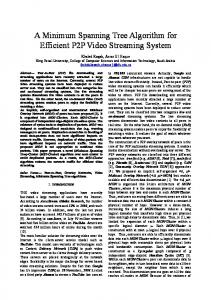
The process is based on constructing a larger data structure OS;, containing records Path;(F’), for every fragment F’ at distajce i of less from F (where distance is measured in F ) . This time, however, once D S ; ( F ) is determined a t r ( F ) ,it also identifies the last node in F on the path to each fragment F’, and appoints it as the node “responsible” for that fragment. In order to set the stage for the (i 1)st iteration of the process, we do the following. The root r ( F ) broadcasts OS; on T ( F ) as before. However, now every node v E F that is responsible for some fragments in the vicinity, sends D S ; ( F ) over the external link to the other end. Since this is done in every fragment, nodes in F adjacent to neighboring fragments F‘ get the data structure D S ; ( F ’ ) , and consequently learn of fragments at distance i+ 1 from F in B. This information can now be used by the nodes in charge to compile their initial suggestions for Path;+l(F‘) for all the new fragments F’ they learn of. The convergecast is again executed and, as in the first iteration, competing candidate paths are eliminated at any vertex along the way during the pipelining. The criterion for elimination is the following. When two paths (of length i), both leading from F to the same fragment F’, compete with each other, we throw away the path that contains the edge with maximum weight in the detected cycle (composed of the two paths combined). Again, the heaviest edge is marked “unusable”. Example: Consider the fragments F and F’ illustrated in Figure 6. Thes? fragments are at distance 2 in the fragment graph F . This fact is discovered in the second phase of the algorithm by the nodes v1 and v2 in F , who identify a length-2 path to F’. The convergecast process on the tree T ( F ) will recognize the fact that there are two paths, and that the edge (211, u1) is the heaviest along the resulting length-4 cycle. Consequently, the path F - F1 - F‘ will be discarded, the sedge ( 2 1 1 , u1) will be marked “unusable”, and the only path to be maintained in D S 2 ( F ) regarding the fragment F’ will be F - F2 - F’. The node responsible for this path in F is 212. I

+

Lemma 3.3 Each node v E F sends to its parent exactly one record P a t h l ( F ’ ) for each fragment F’ that is adjacent t o nodes in U ’ S subtree in T ( F ) ; these records are sent up in increasing order of fragment id. Proof [sketch] The proof is based on showing that at i, a node v on depth L ( v ) = j has already time j received from its descendents all the records concerning paths leading to the ith smallest-id neighboring fragments that are adjacent to vertices in the subtree of T ( F ) rooted at U. This can be proved by double induction (on j and i). I Let F1 be the graph remaining of F after the first iteration (omitting the edges marked “unusable”).

+

Lemma 3.4 If F’ is- a fragment such that d i s t ~ , ( FF’) , = 1, then F1 contains a unique edge connecting F t o F’, and D S 1 ( F )contains the corresponding I record P a t h l ( F , F’). Lemma 3.5 T h e graph

1‘1

contains no parallel edges. Moreover, for every two neighboring fragments F , F’ in the unique remaining edge e in F1 is the lightestweight one.

p,

I

Lemma 3.2 now yields

Coroll_ary 3.6 EF1 contains an MST for the fragment F. I

graph

3.3

Remaining Cycles

In the previous subsection, information is gathered concerning (minimum-weight) paths to neighboring (or, distance 1) fragments. We will be basically repeating this process for 1 phases, eliminating at phase i, 1 5 i 5 I , the inter-fragment cycles of length 2i - 1 and 2i, and keeping minimum-weight paths to distance i fragments. The elimination is performed by throwing away the path containing the edge with maximum weight in the detected cycles. However, the process is more complex than the one described before, and more careful reasoning and pipelining is called for.

3.4

Analysis and Complexity of Part I1

Correctness follows from the _followingclaims. Let F; be the graph remaining of F after the ith iteration (omitting the edges marked “unusable”). By induction on i, we prove the following. Lemma 3.7 If F’ is_ a fragment such that disti;(F, F’) 5 i, then Fi contains a unique path connecting F t o F’, and D S ; ( F ) contains the corresponding I record P a t h ; ( F ,F’).

666

Combined with Lemma 3.8, we get that for 1 = logn, Corollary 3.11 lE(F,)l = O ( N ) .

I

Finally, let us discuss the complexity of performing the short cycle elimination procedure. Each iteration of the cycle elimination phase involves an exchange of DSi-1 over all external links, a convergecast of DSi records and a broadcast of the final picture of DSi from the root. Observe that each record P a i h i ( F ) of DSi consists of O(i1ogn) bits of information, so it can be sent in one time unit. Furthermore, even if each node in F is connected t_o all other existing fragments, there are no more than F records for it to ship upwards, since it forwards a t most one record per adjacent fragment. Since the convergecast is carried out in a fully pipeliced fashion, the i’th iteration requires O(Diam(F)+ilFI)time, and the entire phase I1 takes O ( D i a m ( F ) IF( log2 n) time. By Lemma 2.6, the total running time of this process is bounded as follows.

+

Lemma 3.12 T h e t o t a l running t i m e of P a r t II (short Nlog’n) = O(3’ $+ cycle elimination) is O(d

+

log2n). Figure 6: Cycle Elimination: paths from F to F’ discovered on the second phase (i = 2). The number next to each edge denotes its weight.

4

1. Build a breath-first search tree B on G, the original graph;

2. from every fragment’s center r ( F ) , upcast the list of (uneliminated) external edges adjacent to F on B ;

Lemma 3.8 Girt_h(ki) > 2i. Moreover, the set of edges {e I e E F , e F i } is identical to the set { e I e is the heaviest edge o n some cycle of length 2i

3. the final computation (elimination of edges) is performed centrally at B’s root, who then broadcasts the resulting M S T to all nodes, over the tree B .

F). I

Lemma 3.2 now yields Corollary 3.9 E(f’i) contains an MST for the fragm e n t graph

F. I

Lemma 4.1 P a r t Ill’s t o t a l running t i m e is bounded by i t s o u t p u t is an MST for G . I

O(+ + D i a m ( G ) ) ,and

We now choose to fix 1 = logn, hence we are able to eliminate all cycles in F, of length 2 log n. We then make use of the following known result in extrema1 graph theory, presented in [B], which provides neartight bounds on the relationship between the girth of a graph and the number of edges it contains.

Proof [sketch] The correctness of the output again follows from Lemma 3.2. Let us now estimate the complexity of this part of the algorithm. From the previous section, the total number of edges to be sent up to the root is bounded by O ( N ) . Also, since B is a BFS tree, its depth is O ( D i a m ( G ) ) . Thus, pipelined, all edges arrive at the root in time O ( N Diam(G)). Broadcasting from the root the final MST will take another O(N D i a m ( G ) ) time. I

+

Lemma 3.10 [B]For every integer r 2 1 and n-vertex, = ( V , E )with Girth(G) 2 T , m 5

in-edge graph G i,l+2/(t--2) + n ,

Part 111: Global Edge Elimination

We now proceed to reduce the total number of edges (to the necessary N - 1). Our method is as follows:

Recall that the girth of a graph G , denoted G i r t h ( G ) , is number of edges in the smallest cycle in G . (A single edge is not considered a cycle of length 2, so Girth(G) 2 3 for every G . )

or less i n

+

I

+

I

667

The Complexity of the Combined Algorithm

B. BollobC. Extrema1 Graph Theory. Academic Press, 1978.

Summarizing the results of the last three sections, the complexities of all three parts of our algorithm are as follows, for the given parameter I specified for the first part:

E. Gafni, Improvements in the time complexity of two message-optimal election algorithms, Proc. 4th Symp. on Principles of Distributed Computing, pp. 175-185, August 1985.

5

Part I: Part 11: Part 111:

R. Gallager, P. Humblet and P. Spira, A distributed algorithm for minimum-weight spanning trees, ACM Tkansactions on Programming Languages and Systems, Vol. 5 ( l ) ,pp. 66-77, January 1983.

31 .0(2&) 3'+ .log2n Diam(G)

+

+

The total time complexity is thus optimized when choosing I such that 3' = S , namely, I = b. In 6 For this choice of I, we get 3' = = nc for E = I n 3 - 0.6131.., which yields a total time complexity of -

+

+

A. V. Goldberg, S. Plotkin, and G. Shannon, Parallel symmetry breaking in sparse graphs, Proc. 19th ACM Symp. on Theory of Computing, May 1987.

' n ' 2 6 ) . Since 2 6 = o(nc'> for any E' > 0, we get a bound of O(Diam(G) on the time complexity. Theorem 1.1 follows. o ( D ~ U ~ ( G )

+

N. Linial, Locality as an obstacle to distributed computing, Proc. 27th IEEE Symp. on Foundations of Computer Science, October 1987.

References [An1

D. Angluin, Local and Global Properties in networks of processors, Proc. 12th Symp. on Theory of Computing, pp. 82-93, 1980.

[Awl

B. Awerbuch, Optimal distributed algorithms for minimum-wieght spanning tree, counting, leader election and related problems, Proc. 19th Symp. on Theory of Computing, pp. 230-240, May 1987.

[AGLP]

B. Awerbuch, A. Goldberg, M. Luby and S. Plotkin, Network decomposition and locality in distributed computation, Proc. 30th Symp. on Foundations of Computer Science, pp. 364-375, October 1989.

[AKP]

B. Awerbuch, S. Kutten, and D. Peleg, Competitive Distributed Job Load Balancing, Proc. 24th ACM Symp. on Theory of Computing, 1992, 571-580.

[APl]

B. Awerbuch and D. Peleg, Network synchronization with polylogarithmic overhead, 31'' IEEE Symp. on Foundations of Computer Science, pages 514-522, October 1990.

[AP2]

B. Awerbuch and D. Peleg, Concurrent online tracking of mobile users, Proc. ACM SIGCOMM Symposium on Communication, Architectures and Protocols, Zurich, Sept. 1991, 221-233.

M. Naor and L. Stockmeyer, What can be computed locally? Proc. S T O C 93.

D. Peleg, Time-optimal leader election in general networks, Journal of Parallel and Distributed Computing, Vol. 8, pp. 96-99, 1990. A. Panconesi and A. Srinivasan, Improved distributed algorithms for coloring and network decomposition problems, Proc. 33rd Symp. on Theory of Computing, 1992,581592.

668