Jun 4, 2018 - 3 Test problems with quadratic elements and DG(P2). Sedov. Polar Sod ... We will present a new method to ensure stable mesh motion on shock driven flows using quadratic elements ..... general unstructured grids. Journal of ...
A subcell method for stable mesh motion with Lagrangian hydrodynamic methods on quadratic elements Nathaniel Morgan
Xiaodong Liu
Donald Burton
Los Alamos National Laboratory
June 4, 2018
N. Morgan (LANL)
Lagrangian DG
June 4, 2018
1 / 29
Overview 1
Introduction Governing equations Research background
2
Discretization Modal discontinuous Galerkin (DG) method Multidirectional approximate Riemann solver (MARS) Reducing spurious motion in high-order elements
3
Test problems with quadratic elements and DG(P2) Sedov Polar Sod Isentropic flow Taylor Green vortex
4
Conclusions N. Morgan (LANL)
Lagrangian DG
June 4, 2018
2 / 29
Introduction
N. Morgan (LANL)
Lagrangian DG
June 4, 2018
3 / 29
The goal is to accurately solve the governing evolution equations for Lagrangian hydrodynamics Variables Specific volume Density Velocity Stress Specific total energy Position
Specific volume evolution ρ dv dt = ∇ · u Velocity evolution ρ du dt = ∇ · σ Specific total energy evolution ρ dτ dt = ∇ · (σ · u) Position evolution dx dt = u
N. Morgan (LANL)
v ρ = 1/v u σ τ x
Derivatives d dt
moves with the flow ∇ is in the current coordinate system x Lagrangian DG
June 4, 2018
4 / 29
We seek to create a robust, high-order Lagrangian discontinuous Galerkin (DG) hydrodynamic method The DG method evolves a polynomial Pn forward in time as a function of surface fluxes that come from a Riemann solver and volume integrals. The inputs to the Riemann solver come from the polynomial Pn The DG(P0 ) method is the 1st order accurate FV CCH method Jia et al. [4] and Vilar et al. [8, 9] developed total Lagrangian DG hydrodynamic methods for 2D gas dynamics Vilar et al.[9] developed a 3rd order accurate DG method for quadratic quadrilateral elements, which have edges that bend Morgan et al.[7] developed a velocity filter for reducing spurious mesh motion for DG and FV CCH methods on quadratic elements
The research focus We will present a new method to ensure stable mesh motion on shock driven flows using quadratic elements N. Morgan (LANL)
Lagrangian DG
June 4, 2018
5 / 29
Discretization
N. Morgan (LANL)
Lagrangian DG
June 4, 2018
6 / 29
A total Lagrangian DG formulation will be derived η Volume Ω
Area normal Λs ξ Mapping
Mapping
x = Φ(ξ , t)
Reference element
X = Φ(ξ , t o ) Area normal
Volume, w(t)
an
Mapping
x = Π(X, t) Area normal AN y
Volume V0
Y
x Lagrangian cell at time=t and t>to
X Initial configuration, time=to
Figure: The maps are illustrated for a quadratic quadrilateral element N. Morgan (LANL)
Lagrangian DG
June 4, 2018
7 / 29
The modal DG method is a cell-centered method
The modal DG method approximates fields with Taylor expansions, which creates a very compact numerical stencil The velocity gradient, specific volume, velocity, and specific total energy expansions are L(ξ, t) = ψ (ξ) · Lk (t) v (ξ, t) = ψ (ξ) · v k (t) u(ξ, t) = ψ (ξ) · uk (t) τ (ξ, t) = ψ (ξ) · τ k (t)
N. Morgan (LANL)
Lagrangian DG
June 4, 2018
8 / 29
The modal DG method is a cell-centered method 1 ξ − ξcm η − ηcm ! R 1 1 2 2 ρ(ξ − ξcm ) dw 2 (ξ − ξcm ) − m ψ= w (t) ! R 1 1 2 2 ρ(η − ηcm ) dw 2 (η − ηcm ) − m w (t) R (ξ − ξ )(η − η ) − 1 ρ(ξ − ξ )(η − η )dw cm cm cm cm m
w (t)
k v =
vcm ucm ∂v ∂u ∂ξ cm ∂ξ cm ∂u ∂v ∂η cm ∂η cm k 2 2 u = ∂ v ∂ u2 ∂ξ 2 cm ∂ξ cm ∂2u ∂2v ∂η2 cm ∂η 2 cm ∂2v ∂2u
∂ξ∂η cm N. Morgan (LANL)
∂ξ∂η cm
Lagrangian DG
k τ =
τcm ∂τ ∂ξ cm ∂τ ∂η cm 2 ∂ τ ∂ξ 2 cm ∂2τ ∂η 2 cm ∂2τ
∂ξ∂η cm
June 4, 2018
9 / 29
Nodal quantities are calculated using the Taylor expansions
The pressure, density, and specific internal energy are calculated at the Gauss quadrature points and the element corners η Gauss points g
Corner c Volume Ω
Area normal Λs ξ
Figure: A reference element is shown for a quadratic quadrilateral.
N. Morgan (LANL)
Lagrangian DG
June 4, 2018
10 / 29
The DG approach creates a system of equations to temporally evolve the Taylor coefficients dU =∇·H dt � � Z dU − ∇ · H dw = 0 ψ ρ dt ρ
w (t)
Z
dUk ρψψdw · = dt
w (t)
M·
Z ψ∇ · Hdw w (t)
dUk = dt
Z
ψ∇ξ · (jJ−1 · H)dΩ
Ω
M·
dUk dt
I s · ψjJ
=
−1
∗
· H dΛ −
∂Ω N. Morgan (LANL)
Z
(∇ξ ψ) · jJ−1 · HdΩ
Ω Lagrangian DG
June 4, 2018
11 / 29
A Riemann problem is solved at the element surface nodes p
Riemann force by B. Despr´es and C. Mazeran [3]
z c
y
ai ni
x
F∗c = −pc∗ ac nc = � −pc ac nc + ac µc u∗p − uc · nc nc Riemann force by Maire et al. [6, 5]
Corner 4
Corner 1
F∗i = −pi∗ ai ni = � −pc ai ni + ai µc u∗p − uc · ni ni Riemann force by Burton et al. [2]
Corner 3
Corner 2
Figure: Multidirectional approximate Riemann solver (MARS) N. Morgan (LANL)
F∗i = ai ni · σ ∗c = � ˆc | u∗p − uc ai ni · σ c + µc |ai ni · e The nodal Riemann velocity is found by X F∗i = 0 i∈p Lagrangian DG
June 4, 2018
12 / 29
Spurious motion can arise with high-order elements The density calculated on the subcell should be in agreement with the density field that is evolved using the DG method Spurious motion at the nodes in the middle of the face can be reduced using a subcell density subcell volume, wq(t)
Mq0 ρq = wq δρq = ρq −
y
1 v (ψ q )
ρc = ρc + δρq
x
Figure: Subcell nomenclature
The new method is a higher-order extension of the temporary quadrilateral subzonal (TQS) method by Burton [1] N. Morgan (LANL)
Lagrangian DG
June 4, 2018
13 / 29
Test problems with quadratic elements and DG(P2)
N. Morgan (LANL)
Lagrangian DG
June 4, 2018
14 / 29
The Sedov blast wave test problem
Setup Initial conditions outside source ρ0 = 1 u0 = 0 e0 = 0
1.2
Initial conditions of the source element at the origin 1.2
Figure: Sedov has an energy source in the element at the origin at t=0
N. Morgan (LANL)
ρ0 = 1 u0 = 0 Me 0 = 0.983674/4 γ = 7/5
Lagrangian DG
June 4, 2018
15 / 29
A long standing challenge is that spurious mesh motion arises on strong shock calculations with high-order elements e.g., Sedov
Figure: Spurious mesh motion arises with quadratic quadrilateral elements (resolution = 30x30, γ = 1.4). We developed methods to remove these errors. N. Morgan (LANL)
Lagrangian DG
June 4, 2018
16 / 29
The subcell method with DG(P2) is quite accurate
Sedov Q8 elements (DGP2) 6
Calculation Analytic
5
Figure: The Sedov DG(P2) mesh with quadratic quadrilateral elements (γ = 1.4) and 30x30 resolution
density [g/cc]
4
3
2
1
0
N. Morgan (LANL)
Lagrangian DG
0
0.2
0.4
0.6 position [cm]
0.8
1
June 4, 2018
1.2
17 / 29
The polar Sod test problem
The contact is located at r = 0.5. The initial left state is (ρ0 , ur0 , uθ0 , p 0 )L = (1, 0, 0, 1) The initial right state is (ρ0 , ur0 , uθ0 , p 0 )R = (0.125, 0, 0, 0.1). Calculations will be performed using high-order quadrilateral meshes
N. Morgan (LANL)
Lagrangian DG
June 4, 2018
18 / 29
The polar Sod results are very accurate
Sod Q8 elements (DGP2)
1
density [g/cc]
0.8
0.6
0.4
0.2
0
Figure: The polar Sod DG(P2) mesh with quadratic quadrilateral elements where the resolution is 2 angular elements and 100 radial elements N. Morgan (LANL)
0
0.2
0.4 0.6 position [cm]
0.8
1
Figure: The polar Sod DG(P2) results using the subcell method are in excellent agreement with the analytic solution using a 2x100 resolution
Lagrangian DG
June 4, 2018
19 / 29
The isentropic flow results are very favorable γ = 3 x ∈ [0, 1] ρ0 (x) = 1 + 0.995sin(πx) u0 = 0 p 0 (x) = ρ0 (x)γ
Initial conditions:
Isentropic smooth flow -1
-2
-2
-3
-3 Log(L2-error)
Log(L2-error)
Isentropic smooth flow -1
-4 -5 -6
-8 0.001
0.01 h
-5 -6
DG(P1) DG(P2) 2nd order 3rd order
-7
-4
DG(P1) DG(P2) 2nd order 3rd order
-7
0.1
(a) Density
-8 0.001
0.01 h
0.1
(b) Velocity
Figure: High-order convergence is achieved with DG(P2) and the subcell method N. Morgan (LANL)
Lagrangian DG
June 4, 2018
20 / 29
The Taylor Green (TG) vortex test problem Taylor Green Vortex, zones=202, exact, t=0 1
0.8
0.6
Setup
0.4
Gamma law gas, γ = 7/5 Initial conditions
0.2
0 0
0.2
0.4
0.6
0.8
1
ρ0 ux0 uy0 p0
(a) t=0 Taylor Green Vortex, zones=202, exact, t=1 1
0.8
0.6
= 1 = sin(πx)cos(πy ) = −cos(πx)sin(πy ) = 14 [cos(2πx) + cos(2πy )] + 1
Energy source term
0.4
0.2
Sτ = 0 0
0.2
0.4
0.6
0.8
π 4(γ−1) [cos(3πx)cos(πy )
−cos(3πy )cos(πx)]
1
(b) t=0.75 Figure: The TG vortex exact solution N. Morgan (LANL)
Lagrangian DG
June 4, 2018
21 / 29
TG vortex results are very accurate Taylor Green Vortex, zones=152, exact, t=0.75 1
0.8
0.6
0.4
0.2
0 0
0.2
0.4
0.6
0.8
1
(a) Exact solution
(b) DG(P2) with subcell method
Figure: The Taylor-Green vortex results at t=0.75 using DG(P2) and higher-order quadratic elements (15x15 resolution). The subcell method delivers high-order accuracy and improved mesh stability. N. Morgan (LANL)
Lagrangian DG
June 4, 2018
22 / 29
TG vortex results are very accurate Taylor-Green vortex at t=0.1 -1.5 -2 -2.5
Log(L2-error)
-3 -3.5 -4 -4.5 Simpson Sub-cell 2nd order
-5 -5.5
3rd order -6
0.01
0.1 h
Figure: High-order convergence is achieved on the Taylor-Green vortex problem using DG(P2) with the subcell method. N. Morgan (LANL)
Lagrangian DG
June 4, 2018
23 / 29
Conclusions
N. Morgan (LANL)
Lagrangian DG
June 4, 2018
24 / 29
Summary We presented a new subcell method that produces stable and accurate mesh motion with a Lagrangian DG(P2) hydrodynamic method using quadratic elements Results on the Sedov and polar Sod test problems were very accurate and the mesh deformed in a stable manner 3rd-order accuracy was achieved on the isentropic flow and the Taylor-Green vortex test problems
Figure: A movie of the Gresho vortex to t=1 using the DG(P2) with the subcell method. N. Morgan (LANL)
Figure: A movie of the Taylor Green vortex to t=1 using the DG(P2) with the subcell method.
Lagrangian DG
June 4, 2018
25 / 29
Acknowledgements
Thank you! We gratefully acknowledge the support of the NNSA through the Laboratory Directed Research and Development (LDRD) program at Los Alamos National Laboratory. The Los Alamos unlimited release number is LA-UR-18-24668. Los Alamos National Laboratory is operated by Los Alamos National Security, LLC for the U.S. Department of Energy NNSA under Contract No. DE-AC52-06NA25396.
N. Morgan (LANL)
Lagrangian DG
June 4, 2018
26 / 29
References I [1] D. Burton. Temporary quadrilateral subzoning. Technical report, Lawrence Livermore National Laboratory, 1992. [2] D. Burton, T. Carney, N. Morgan, S. Sambasivan, and M. Shashkov. A cell-centered Lagrangian Godunov-like method of solid dynamics. Journal of Computers & Fluids, 83:33–47, 2013. [3] B. Despr´es and C. Mazeran. Lagrangian gas dynamics in two dimensions and Lagrangian systems. Arch. Rational Mech. Anal., 178:327–372, 2005. [4] Z. Jia and S. Zhang. A new high-order discontinuous Galerkin spectral finite element method for Lagrangian gas dynamics in two-dimensions. Journal of Computational Physics, 230:2496–2522, 2011. N. Morgan (LANL)
Lagrangian DG
June 4, 2018
27 / 29
References II
[5] P-H. Maire. A high-order cell-centered Lagrangian scheme for two-dimensional compressible fluid flows on unstructured mesh. Journal Computational Physics, 228:2391–2425, 2009. [6] P-H. Maire, R. Abgrall, J. Breil, and J. Ovadia. A cell-centered Lagrangian scheme for two-dimensional compressible flow problems. SIAM Journal Scientific Computing, 29:1781–1824, 2007. [7] N. Morgan, X. Liu, and D. Burton. Reducing spurious mesh motion in Lagrangian finite volume and discontinuous Galerkin hydrodynamic methods. Accepted to Journal of Computational Physics, 2018.
N. Morgan (LANL)
Lagrangian DG
June 4, 2018
28 / 29
References III
[8] F. Vilar. Cell-centered discontinuous Galerkin discretization for two-dimensional Lagrangian hydrodynamics. Computers & Fluids, 64:64–73, 2012. [9] F. Vilar, P-H. Maire, and R. Abgrall. A discontinuous Galerkin discretization for solving the two-dimensional gas dynamics equations written under total Lagrangian formulation on general unstructured grids. Journal of Computational Physics, 276:188–234, 2014.
N. Morgan (LANL)
Lagrangian DG
June 4, 2018
29 / 29