European Congress on Computational Methods in Applied Sciences and Engineering ECCOMAS 2004 P. Neittaanm¨ aki, T. Rossi, K. Majava, and O. Pironneau (eds.) W. Rodi and P. Le Qu´ er´ e (assoc. eds.) Jyv¨ askyl¨ a, 24–28 July 2004
VORTEX METHOD WITH FULLY MESH-LESS IMPLEMENTATION FOR HIGH-REYNOLDS NUMBER FLOW COMPUTATIONS L. A. Barba? , Anthony Leonard† , and C. B. Allen? ? Department
of Aerospace Engineering University of Bristol, Queen’s Bldg., University Walk, Bristol, U.K. BS8 1TR e-mails:
[email protected],
[email protected] †
Graduate Aeronautical Laboratories California Institute of Technology, Pasadena, CA 91125, U.S.A. e-mail:
[email protected]
Key words: vortex methods, mesh-less CFD, viscous vortices, core spreading, radial basis functions. Abstract. A new viscous vortex method has been developed, where the mesh-less character of the method is preserved throughout. Many vortex methods use a particle strength exchange (PSE) scheme for viscous effects, and remeshing processes with high-order interpolation kernels to maintain an ordered particle field. In the present work, diffusion is accounted for using the core spreading scheme, and spatial adaption is provided in a mesh-less formulation using radial basis function interpolation. Core size control is effected automatically in the spatial adaption process, and thus convergence is assured. This method has been demonstrated to provide significant increase in the accuracy of computations with Lagrangian vortex particles. Furthermore, the combination of core spreading and RBF-based spatial adaption allows an implementation with variable resolution, and multi-scale computation are practicable as well. Presently, proof-of-concept computations are presented of a flow consisting of a Gaussian monopole with a localized elliptic deformation, which evolves with a quasi-steady state consisting of a rotating tripole. The new method has been implemented in parallel, and thus highly accurate computations of viscous vortex interactions have been practicable. Results are presented where calculations of the early interaction of two co-rotating vortices compare extremely well with published results using spectral methods. 1
L. A. Barba, Anthony Leonard and C. B Allen
1
INTRODUCTION
The traditional methods of CFD, such as finite volumes and finite elements, are dependent on the construction of a good-quality mesh on the domain of computation. Not only is mesh generation a time-consuming, expensive process of CFD, but the Eulerian and grid-dependent computational methods suffer inevitably from numerical diffusion. In some instances, such as when computing flows at high-Reynolds numbers with concentrated areas of vorticity, numerical diffusion can overwhelm the physical viscous process, and one finds that vortices are not well captured or simply diffuse too fast. On the other hand, spectral methods provide an alternative for high-accuracy calculations, and thus many workers prefer this approach for the computation of viscous vortex interactions at high-Reynolds numbers. Spectral methods, however, are quite limited in the geometries that they can deal with, and in some instances a very large computational domain is necessary to minimize the effects of periodic images. An alternative to conventional grid-dependent CFD methods is the Lagrangian vortex method, which is formulated without a need for connectivity of the computational elements. This method utilizes vortex particles as the computational units, and these are convected with the local fluid velocity to solve the vorticity transport equation. Thus, the non-linear term of the Navier-Stokes equations is translated into a system of ODE’s for the trajectories of the vortex particles, and there are no numerically diffusive truncation errors. Furthermore, the method has no CFL-like stability constraints. The diffusion of vorticity is implemented in vortex methods in a variety of ways: stochastically, by adding Brownian-like motion to the particles (random vortex method, RVM), or deterministically, by changing the particle circulation strengths, vorticity distribution, size or location such that the diffusive part of the Navier-Stokes equation is satisfied. Thus, vortex methods provide an attractive alternative for computing flows at high-Reynolds numbers. Over the years, a number of reviews have been published describing the developments in vortex methods [1, 2, 3, 4, 5], and recently a book has been dedicated to the subject [6]. Convergence of vortex methods under different assumptions has been proved in [7, 8, 9, 10, 11], and in [12] including time-stepping. The Lagrangian formulation in vortex methods has encountered some difficulties, however. First, with the introduction of high-order spatial discretizations [13], it was found that the accuracy was very quickly lost as the particles convect, and hence ‘rezoning’ strategies were introduced. Second, with the application of general particle methods [14] to formulate a viscous scheme in terms of integral operators (particle strength exchange, PSE), the use of quadratures on the particle locations to compute the integrals meant that accuracy relied on nearly regular particle distributions. Thus, ‘remeshing’ schemes were developed [15, 16]. Vortex methods with PSE and remeshing have been used with considerable success to simulate separated flows around bluff-bodies [17, 18, 19, 20] and also in computations of fundamental processes in vortex dynamics, such as axisymmetrization [21]. Some authors, nevertheless, have been concerned that the use of remeshing schemes
2
L. A. Barba, Anthony Leonard and C. B Allen
—which due to their formulation in terms of tensor products require the construction of a Cartesian mesh for the new particle locations— cripples the vortex method with a mesh. Indeed, a new algorithm for viscosity was developed with the sole goal of avoiding remeshing, namely, the vortex redistribution method [22]. On the other hand, one may legitimately expect that the mesh-based interpolation used in remeshing introduces some numerical diffusion. Numerical experiments were performed recently by the authors [23] where the effects of remeshing were considered. Using classic test problems that possess an analytical solution, such as inviscid vortex patches and the Lamb-Oseen vortex, time-marching experiments with remeshing showed that, with a very accurate initialization, the first remeshing event produced a large jump in the errors. Similar results will be presented here to argue that standard remeshing schemes, although they allow for long-time calculations, do introduce noticeable interpolation errors. To avoid the shortcomings of remeshing, in this work a method has been developed where spatial adaption is formulated using radial basis function (RBF) interpolation, a mesh-less scattered data interpolation technique. This method has received significant attention in the past years in the function approximation community, and it will be briefly presented in §3, after introducing the general formulation of the vortex method in §2. The vortex method implemented in this work uses core spreading for diffusion. As discussed further below, this method has many attractive features, but requires some form of core size control to ensure convergence. This will be provided by the mesh-less spatial adaption process in a straightforward way. In §4, a brief presentation of numerical experiments using classic test problems will demonstrate the need for spatial adaption in vortex methods —regardless of the viscous scheme used—, and the accuracy limitations imposed by the standard remeshing schemes. The potential of overcoming this limitation with the mesh-less spatial adaption based on RBF interpolation is discussed in §3. Some of this progress was previously presented in [23]. Applications to flows of real fluid dynamical interest will be demonstrated in §6. The first application corresponds to the evolution of a Gaussian monopole with a quadrupolar perturbation, resulting in a localized elliptical deformation. This flow presents a quasisteady state in the form of a rotating tripole, and was previously studied in [24] using a vortex method with core spreading and particle splitting. Our results agree well with those of [24], in general, but are noticeably smoother. In addition, where for the lower Reynolds number case calculated in [24] the tripole structure erodes, we still obtain a tripole in this case. We argue that the difference is accountable to the numerical diffusion introduced in the particle splitting scheme. The second application corresponds to the early interaction of two co-rotating vortices, when they both adapt to each other’s strain field by acquiring an elliptical deformation of the core and small-scale azimuthal perturbations. This flow was recently studied in [25], where it was computed using spectral methods; we obtain a remarkable agreement with 3
L. A. Barba, Anthony Leonard and C. B Allen
those results, even at a vorticity level as weak as ∼ 10−6 . Thus, this is a very exacting test for any numerical method, and demonstrates that high-accuracy can be achieved with a completely mesh-less vortex method. 2
GENERAL FORMULATION OF THE NUMERICAL METHOD
The governing equation in vortex methods is the vorticity transport equation, obtained by taking the curl of the momentum equation. Assuming incompressible flow, and for the two-dimensional case, this is: ∂ω + u · ∇ω = ν∆ω (1) ∂t where ω(x, t) = ∇ × u(x, t) represents the vorticity field, which becomes the principal variable for computation (note that the pressure is absent from the formulation). The vortex method proceeds by discretizing spatially the vorticity field using elemental vortices, which are characterized by a distribution of vorticity, ζσi (commonly called the cutoff function), a circulation strength Γi , a core size σi , and a spatial location xi . Thus, the discretized vorticity is expressed by: h
ω(x, t) ≈ ω (x, t) =
N X
Γi (t)ζσi (x − xi (t)) .
(2)
i=1
It is the usual case that the core sizes are uniform (σi = σ), and the cut-off function is frequently a Gaussian distribution; the following was used in this work: µ ¶ −|x|2 1 ζσ (x) = exp . (3) 2πσ 2 2σ 2 The velocity field is obtained from the vorticity by means of the Biot-Savart law: Z Z 0 0 0 u(x, t) = (∇ × G)(x − x )ω(x , t)dx = K(x − x0 )ω(x0 , t)dx0 = (K ∗ ω)(x, t) where K = ∇ × G is the Biot-Savart kernel, with G the Green’s function for the Poisson equation, and ∗ representing convolution. The vorticity transport is solved in this discretized form by convecting the particles with the local fluid velocity, and accounting for viscous effects by changing the particle vorticity. Hence, the unbounded vortex method is expressed by the following system of equations: dxi = u(xi , t) = (K ∗ ω)(xi , t), dt
dω(xi , t) = ν∇2 ω(xi , t). dt
(4)
The viscous contribution is provided in this work by applying the core spreading method [26, 1], where the elemental vortices are allowed to grow in time to solve the diffusion equation exactly. In this method, one can view the discretized vorticity field as a superposition 4
L. A. Barba, Anthony Leonard and C. B Allen
of “spreading line vortices” (see Batchelor [27], p. 204) of different circulation strengths Γi . Hence, to satisfy identically the viscous part of the vorticity equation when using the cutoff given in (3), one lets σ 2 grow linearly according to dσ 2 = 2ν. dt
(5)
Thus, the method is expressed in the following simple algorithmic rule: σi2 (t + ∆t) = σi2 (t) + 2ν∆t,
i = 1···N
(6)
The core spreading method has the advantages of being fully localized and grid-free, and deterministically solving the diffusion of vorticity. As implied in (6), it can easily deal with variable core sizes in the domain. Its use, however, effectively stalled when consistency issues were raised in [28]. The method was shown to converge to an equation that differs from the Navier-Stokes equation in the convection term, by transporting the vortex elements with an averaged velocity. The consistency error of core spreading is caused by the advection without deformation of larger and larger vortex blobs as they spread. A solution to this problem by means of a scheme for splitting the elemental vortices was finally proposed in [29], where linear convergence of the corrected method was proved. The numerical experiments presented in [29], however, reveal that the method with blob splitting can be compared in accuracy with the random vortex method (RVM). Indeed, in a case using a Lamb-Oseen vortex, plotted results of the calculated tangential velocity show quite visible errors. Other experiments shown were directly compared to the RVM; it should be noted, however, that the Reynolds number chosen (Re = 100) is near the lower-limit of acceptability of the RVM. It would seem, then, that the proposed splitting scheme is of rather low accuracy. Alternative splitting formulae were studied in [30], and an empirical rule for determining the splitting ratio α, determining the size of the children particles as ασ, was developed. Nevertheless, the scheme was not able to improve on results using PSE with standard remeshing. Presently, core size control to ensure convergence of the core spreading will be provided automatically in the RBF interpolation used for spatial adaption, without the need to apply particle splitting. 3
RADIAL BASIS FUNCTION INTERPOLATION
Radial basis function (RBF) methods are techniques for interpolation or approximation of multi-variate functions, which have received considerable attention from the function approximation community in recent years. A brief survey of recent developments can be found in [31], and also a book has been published very recently on the subject [32]. These techniques were originally developed for the interpolation of topographic data, in [33] the two-dimensional multi-quadric (MQ) functions are derived and used to approximate geographical surfaces, whereas the thin-plate spline (TPS) functions are derived in [34] and also [35, 36]. They remained rather obscure until reviewed in [37], where nearly 30 different 5
L. A. Barba, Anthony Leonard and C. B Allen
algorithms for scattered data interpolation were tested and compared, using a variety of criteria. Global basis functions were ranked best in this survey, which brought about much interest and further research. The use of RBF techniques for numerical solution of partial differential equations was introduced in [38, 39], where MQ’s provided the spatial discretization scheme. They have also found application in artificial intelligence, such as learning from examples [40], and they have been used with remarkable results in geometric modelling [41]. In [42] their use for interpolation of the information between unstructured grids is demonstrated, which is similar to our application. The problem of scattered data interpolation is that of how to approximate an unknown function f ∈ C(Ω) whose values are known on a set X = {x1 , . . . , xN } ⊂ Ω ⊂ Rd . The RBF approach, where we follow the notation of [43], is to choose the function that approximates f to be of the form: sf,X (x) =
N X
αj Φj (x, xj ) + p(x),
(7)
j=1
where p(x) is a low-degree polynomial, and Φ : Ω × Ω → R is the basis function; it is simpler numerically to deal with bases that are translation invariant, an in particular those that satisfy: Φ(x, y) = φ(kx − yk2 ) with φ : [0, ∞) → R (radiality)
(8)
Clearly, the vortex blob discretization of the vorticity is analogous to the interpolant (7), where the polynomial part is chosen as null and the basis function is the cutoff function, a Gaussian for example. Indeed, Gaussians are used in RBF interpolation (and usually with null polynomial part), as are basis functions of the following types: (i) (ii) (iii)
φ(r) = rβ , β > 0, β ∈ / 2N : ‘pseudo-cubics’ 2k φ(r) = r log(r), k ∈ N : ‘thin-plate splines’ φ(r) = (c2 + r2 )β , β > 0, β ∈ / N : ‘multi-quadrics’
(9) (10) (11)
The solution of (7) requires the satisfaction of the interpolation conditions by collocation, leading to a linear system for the coefficients α = (α1 , . . . , αN ) and the polynomial coefficients. For our purposes, we can assume that the polynomial part is null, and write the system as: Φα = f~ (12) where f~ represents the vector of function values at the centres, f~ = {f (x1 ), . . . , f (xN )}, and Φij = φ(kxi − xj k). The matrix Φ being full and not well conditioned, Franke [37] concluded that global basis function methods are not feasible for large N . But since then, a great deal of work has contributed to effectively resolve this and several other difficulties. Preconditioning operators were first introduced in [44] for the cases of the MQ and TPS, 6
L. A. Barba, Anthony Leonard and C. B Allen
based on triangulation of the data points and construction of discrete approximations to the iterated Laplacian operators, ∆k . At the same time, theoretical progress was made, with the result of [45] that the interpolation system (12) is guaranteed a solution whenever the function Φ(x, y) is strictly conditionally positive definite and the data distinct. As described in [43] (where proofs are given), the theory has been greatly extended and many basis functions have been characterized, for example, the MQ interpolant is conditionally positive definite and can be made positive definite by appending a linear polynomial, and the Gaussian is positive definite hence not requiring a polynomial part. Significant progress has been made in regards to computational efficiency of RBF methods. Evaluating a function whose approximation has been expressed as an expansion in RBFs can be quite expensive, involving O(N ) operations for each evaluation point. Multipole expansions for the fast evaluation of the interpolant (7) were introduced for the TPS in [46], where in addition the fast algorithms are also applied to the matrix-vector product required at each step of an iterative solution method, in particular the pre-conditioned conjugate-gradient method. A new method for the fast evaluation of RBF expansions, based on generalizing the multipole method so that changes of basis are easily performed, was presented in [47]. In addition, the actual solution of the RBF interpolation problem can be prohibitive for large N , unless fast methods are implemented. This was successfully addressed in [48], where preconditioning strategies were used in conjunction with fast matrix-vector multiplication and a GMRES iterative solution method. Alternatively, an approach for the fast solution of RBF interpolation analogous to forward substitution is developed in [49, 50], based on generalization of the iterative method constructed in [51]; this was applied to TPS while the extension to the MQ and other conditionally positive definite functions was shown to be accessible. Considerable improvements to this method have been performed, in particular the inclusion of a Krylov subspace algorithm which is guaranteed to converge [52]. A third approach for the efficient solution of the RBF interpolation system is based on domain decomposition [53]; such a method was applied to data sets of up to 5 million two-dimensional points. 4
ACCURACY OF THE VORTEX METHOD AND STANDARD REMESHING SCHEMES
One of the early efforts to analyze and quantify the accuracy of vortex methods [54] recognized the fundamental importance of three factors: the way an existing/initial vorticity field is discretized/initialized, the choice of cutoff function used, and the value of the cutoff parameter, σ. The numerical experiments presented in [54] showed that for σ ≈ h, where h is the initial inter-particle spacing, the accuracy at initialization was deteriorated quite quickly. It was proposed then that the optimal choice of σ be made in function of the final time desired for the computation (i. e., by providing an initially denser particle field when longer calculations were desired). This suggestion does not consider the possible application of some form of spatial adaption. With effective spatial adaption, one may perform considerably longer calculations. 7
L. A. Barba, Anthony Leonard and C. B Allen
−1
−1
10
10
−2
−2
10
10
−3
−3
10
10
−4
−4
10
10
−5
−5
10
10
−6
−7
10
2
−6
velocity, L2−norm vorticity, L2−norm velocity, max. rel. vorticity, max. rel.
10
2.2
2.4
2.6
2.8
3 time, t
3.2
3.4
3.6
3.8
velocity, L2−norm vorticity, L2−norm velocity, max. rel. vorticity, max. rel.
10
−7
4
10
2
2.2
2.4
2.6
2.8
3 time, t
3.2
3.4
3.6
3.8
4
(b) M40 remeshing every 10 time-steps.
(a) No remeshing.
Figure 1: Lamb-Oseen vortex test; Gaussian blobs σ = 0.025, h/σ = 0.7 and N = 2177, ∆t = 0.02.
The loss of accuracy in the vortex method due to the Lagrangian distortion of the initial particle field is demonstrated in Figure 1(a), where the measured errors in a calculation using a Lamb-Oseen vortex are shown as they evolve in time. The vortex has initial circulation Γ0 = 1.0, and the Reynolds number based on the circulation, Re = Γ0 /ν is 1000. The initial time is chosen as t0 = 2.0 for a vorticity distribution given by: ω(|x|, to ) =
|x|2 Γ0 − 4νt o. e 4πνto
(13)
A Runge-Kutta 4th -order method was used for time-stepping, and the numerical parameters are indicated in the figure caption. It can be seen how, without spatial adaption, there is a loss of accuracy of about three orders of magnitude: the L2 -norm velocity error is 2.7 × 10⁻⁷ after the first time step, and it is 6.4 × 10⁻⁴ by the end of 100 time steps. A moderate gain is observed when adding a standard remeshing scheme, in this case using the so-called M40 interpolation kernel, introduced in [55] (see [21] or [6], p. 229), velocity errors decrease by about 50%. This is just one example of a large number of numerical experiments where the same overall behavior was observed: without spatial adaption the errors grow considerably, but not without bound; adding standard remeshing, errors are diminished (in most cases, by about one order of magnitude) but most of the loss of accuracy occurs on the first remeshing event. This ‘initial remesh error’ reveals that the standard mesh-based spatial adaption scheme limits the accuracy of the vortex method. Note that the usual diagnostics used for assessing the performance of remeshing schemes, namely, the conservation of total circulation and of linear impulse, indicate that the schemes are successful. For example, 8
L. A. Barba, Anthony Leonard and C. B Allen
−1
10
M’4 REMESHING
−2
10
−3
10
−4
10
−5
10
−6
10
RBF−spatial adaption
−7
10
velocity, L2−norm vorticity, L2−norm velocity, max. rel. vorticity, max. rel.
−8
10
−9
10
2
2.2
2.4
2.6
2.8
3 time, t
3.2
3.4
3.6
3.8
4
Figure 2: Lamb-Oseen vortex test; Gaussian blobs, σ = 0.025, h/σ = 0.7 and N = 2177, ∆t = 0.01. M40 remeshing and RBF-based spatial adaption with SOR every 10 steps.
in the example of Figure 1(b), the maximum change in total circulation was 3.66 × 10⁻¹⁵ and the maximum change in x-impulse was 2.51 × 10⁻¹⁷ . 5
SPATIAL ADAPTION WITH RBF INTERPOLATION
In Figure 2 is shown a plot of the evolution of errors when the Lamb-Oseen vortex test with remeshing shown previously was repeated using a smaller time step. This results in smaller errors during the early part of the calculation, but evidences a much larger jump due to ‘initial remesh error’. On the same plot is shown the result of an experiment performing RBF interpolation to obtain the new, spatially-adapted, set of particles (which were placed on a square lattice, for simplicity) . Both results are shown with the same line styles, but they are easily discernible because the difference in accuracy is between three and four orders of magnitude. The RBF interpolation is obtained by first calculating the vorticity value on each location for the new particles, induced by the set of old particles, and then solving the RBF system (12) for the new particle strengths. In this test, a successive over-relaxation method was used, with a parameter % = 0.4 (under-relaxation) and an imposed maximum number of 100 iterations. This method of solution was chosen on the first instance because it had previously been applied to obtain an accurate initialization of a vortex method calculation in [21]. The under-relaxation parameter had to be chosen by trial and error, which is one of the draw-backs of the method of SOR. Subsequently to the initial successful tests, other methods of solution have been implemented. In these tests using the Lamb-Oseen vortex, diffusion was accounted for using the core spreading method. Without any spatial adaption, or when using standard remeshing, the 9
L. A. Barba, Anthony Leonard and C. B Allen
t=0 6
6
0.3
0.9 0.8 4
4
0.2
2
0.1
0.7 0.6
2
0.5
0 0
0
0.4 0.3
−0.1 −2
−2
0.2
−0.2
0.1 −4
−4
0
−0.3 −0.1 −6 −6
−4
−2
0
2
4
−6 −6
6
(a) Total vorticity.
−4
−2
0
2
4
6
(b) Perturbation vorticity.
Figure 3: Initial condition for the perturbed monopole calculations, normalized by ωo,max .
cores continue to grow until the end of the computation, in the cases shown in Figure 1, from σ0 = 0.025 to σT = 0.0681 (note that the inconsistency proved in [28] does not apply when there is radial symmetry). When performing the spatial adaption by RBF interpolation, in contrast, it is easy to set the new core sizes to their original value. Upon implementing this form of core size control, the maximum core size in these tests is σmax = 0.0287. Therefore, this method allows core size control for the core spreading without vortex splitting. 6 6.1
APPLICATIONS: COMPUTATION OF VISCOUS VORTEX INTERACTIONS Perturbed Gaussian vortex monopole with tripole attractor
When a two-dimensional monopolar vortex is added a quadrupolar perturbation, the principal effect is an elliptical deformation of the main vortex (Figure 3). One of the relevant questions apropos of two-dimensional vortices with elliptical shapes is whether they decay to an axisymmetric state. The process of ‘axisymmetrization’ is recognized as one of two fundamental processes in the evolution of two-dimensional turbulent flows, the other being vortex merging [56]. These processes participate in the notorious evolution of two-dimensional turbulence to form isolated, ‘coherent’ vortices, that live for many eddy turn-over periods [57]. In [58], the relaxation of linearly perturbed, large Re Lamb-Oseen vortices was studied numerically using finite difference methods, and it was seen that the non-axisymmetric perturbations decay much faster than the viscous time scale. A mechanism of shear-diffusion averaging [59] is active, whereby the shearing along streamlines causes the winding-up of the non-axisymmetric vorticity into spiral structures, which are then rapidly homogenized due to viscous diffusion. In this case, the axisymmetric state 10
L. A. Barba, Anthony Leonard and C. B Allen
is approached on a Re1/3 time scale, as shown in [59]. Fully nonlinear simulations of this flow were presented in [24], where a vortex method is used with core spreading and vortex particle splitting [29]. In that work, it was observed that for large enough amplitudes of the perturbation, the flow relaxes to a quasi-steady, rotating tripole. The shear-diffusion mechanism in this case is still active, but the flow relaxes to the tripole instead of the monopole, as only the positive portions of the perturbation are mixed while the negative parts form persistent inclusions. Thus it was suggested that there exists a threshold amplitude separating the domains of attraction of the monopole and tripole. Tripolar vortices have been observed in experiments [60, 61], and they have also been observed in numerical simulations of evolving turbulence [62]. A vortex tripole was observed by satellite imaging on the Bay of Biscay, surviving for several days [63]. Thus, the tripole is now recognized as one more ‘elemental’ coherent vortical structure of geostrophic and two-dimensional turbulent flow. Presently, the vortex method with mesh-less spatial adaption has been used to compute the evolution of a Lamb-Oseen vortex, with a quadrupolar perturbation of sufficient amplitude, according to the studies of [24], to produce a quasi-steady tripole. Calculations were performed for Reynolds numbers Re = 500, 103 , 5000, 104 . The initial condition is given by the vorticity ωo with perturbation ω 0 , given below: µ ¶ µ ¶ 1 −|x|2 −|x|2 δ 0 2 ωo (x) = exp , ω (x) = |x| exp cos 2θ. (14) 4π 4 4π 4 Figure 4 shows the vorticity field (top row) and the vorticity perturbation (bottom row) at two intermediate and the final times of the calculation, for the case Re = 104 and δ = 0.25. These plots reproduce very well the rotation angle of the structure and shape of contours of the results presented in [24] (Fig. 1, p. 2330), although we obtain smoother contours with sharper fine details. There are no numerical parameters reported in [24], but one of the authors informally stated to us that the computations were in the “low to middle 10’s of thousands” of vortex elements (L. F. Rossi, private communication 2004). Their calculations were performed quite some years ago, and indeed they required a mainframe computer (Cray C90). The present results were obtained on a common desktop PC and the maximum number of particles was N = 4600. Time-stepping was performed with Runge-Kutta of 4th order, with ∆t = 1 and vortex particles were initialized and adapted to a triangular lattice with equivalent resolution on a square lattice given by h = 0.18, and the overlap ratio was h/σ = 0.9. The RBF interpolation system was solved using GMRES, without preconditioning in this case. In Figure 5 are shown three plots of the vorticity perturbation at a time t = 500, for different Reynolds numbers. This corresponds to Fig. 8 (p. 2337) of [24], and it can be seen that once again the present results are much smoother, but more importantly, the general agreement applies only to the two higher values of Re. For Re = 1000 we obtain significant differences with the results of [24], where it was observed in this case that the tripole structure is significantly eroded at t = 500. Our result shows that the perturbation 11
L. A. Barba, Anthony Leonard and C. B Allen
t = 300
t = 450
t = 600
6
6
6
4
4
4
2
2
2
0
0
0
−2
−2
−2
−4
−4
−4
−6 −6
−4
−2
0
2
4
6
−6 −6
−4
−2
t = 300
0
2
4
6
−6 −6
6
4
4
4
2
2
2
0
0
0
−2
−2
−2
−4
−4
−4
−2
0
2
4
6
−6 −6
−4
−2
0
0
2
4
6
2
4
6
t = 600
6
−4
−2
t = 450
6
−6 −6
−4
2
4
6
−6 −6
−4
−2
0
Figure 4: Perturbed monopole relaxing to a tripole attractor. Reynolds number is 104 , strength of the perturbation is δ = 0.25. Top: total vorticity field; 15 equally-spaced positive contours, and 3 equallyspaced negative contours in dotted line. Bottom: perturbation vorticity; 10 equally-spaced contours of each sign (negative contours in dotted line).
t = 500
t = 500
t = 500
6
6
6
4
4
4
2
2
2
0
0
0
−2
−2
−2
−4
−4
−4
−6 −6
−4
−2
0 Re = 1000
2
4
6
−6 −6
−4
−2
0 Re = 5000
2
4
6
−6 −6
−4
−2
0 Re = 10000
2
4
6
Figure 5: Tripole attractor perturbation vorticity at varying Reynolds number: from left to right, Re = 103 , 5000, 104 ; maximum vortex blob core radius, respectively, 0.245, 0.21, 0.205; 10 equally-spaced contours of each sign (negative contours in dotted line).
12
L. A. Barba, Anthony Leonard and C. B Allen
is indeed being decreased in magnitude due to diffusion (as well as the base vortex), but the positive center and the negative inclusions continue to have comparable strength, and the tripole is still clearly visible until the end of the computation. Indeed, we performed a calculation at Re = 500 and the same observation holds: although the perturbation amplitude has decayed, the relative strength of the positive center and negative inclusions is still close to 1. It is our view that the differences observed with the results of [24] for the lower Re case reflect that in the latter case there is numerical diffusion introduced by the vortex particle splitting scheme. In the more viscous calculations, an imposed value for the maximum core size results in particle splitting being performed much more often. Hence, splitting errors accumulate for the low Re case. The implication of our calculations, where the spatial adaption effects core size control automatically without splitting, is that the tripole structure is more persistent than previously thought, and is not eroded at low Re. 6.2
Early interaction of co-rotating vortices
The interaction of two co-rotating vortices is characterized by the fundamental process of vortex merging. For the case of inviscid vortex patches, the interaction is governed by the ‘merger criterion’, which stipulates the critical distance between the vortices under which merging will occur [64]. Above this distance, the vortices exhibit a deformed shape, until when they are sufficiently far apart they maintain their approximately circular shape. In the case of viscous flow, the sizes of the vortices grow with time, so that eventually they will reach the critical distance, and merge [65]. At higher Reynolds numbers, the time necessary to reach the critical distance will be larger, and thus it is possible to observe the early interaction of the vortices in some detail. In the merging process of viscous vortices, different stages have been distinguished [65]. The first is an ‘adaptation’ stage, when each vortex is elliptically deformed due to the strain field produced by the other. This is an important interaction due to the fact that in three dimensions the elliptically deformed vortices are subject to the so-called ‘elliptic instability’ [66, 67, 68]. In the second stage, the vortices are in a ‘metastable state’ and evolve on a viscous time scale. Their distance remains relatively constant, and they rotate around each other at a frequency very close to that of two point vortices of same circulation. In the third stage, the vortices reach their critical state, and finally, they rapidly merge on the convective time scale. The adaptation stage of two viscous co-rotating vortices was studied numerically using spectral methods in [25]. This paper includes a plot of vorticity contours during the early evolution of the vortices at Re = 8 × 10⁴ , showing logarithmic contour levels down to a value of 10−6 . We considered this to be a very exacting test for any numerical method, and set about to reproduce these results with the present vortex method. To this end, the method was implemented in parallel, using the PETSc library in a C++/MPI code. The PETSc library [69] provided the preconditioners and GMRES solution method, used both at initialization and during each RBF spatial adaption process, as well as vector 13
L. A. Barba, Anthony Leonard and C. B Allen
and matrix assembly and manipulation in parallel . With this new implementation of the method, a high-accuracy calculation was performed, with up to 2 × 10⁴ vortex particles. The results, shown in Figure 6, reproduce remarkably well those presented on [25], where a 1024 × 1024 computational mesh was used. Hence, it has been demonstrated that accurate calculations, comparable to those that can be obtained with spectral methods, are possible with the mesh-less vortex method; and indeed, using reduced problem sizes. 7
CONCLUSIONS
This work demonstrates a new viscous vortex method, with a wholly mesh-less formulation. To accomplish high-accuracy, the method implements spatial adaption of the vortex particles using radial basis function (RBF) interpolation. In this way, no logically ordered mesh is required for the spatial adaption process. In addition, the RBF interpolation allows for automatic core size control during the spatial adaption, thereby permitting the use of the core spreading scheme for diffusion and ensuring convergence. The combination of core spreading and RBF interpolation has many advantages, particularly at high Reynolds numbers. Core spreading solves the diffusion equation exactly, and does not suffer from quadrature errors, as is the case in the prevalent method of particle strength exchange. In addition, it is fully localized and grid-free, and hence ‘embarrassingly parallel’. The RBF interpolation, on the other hand, not only preserves the mesh-less implementation of the method, but has high accuracy and allows easily for variable resolution in the physical domain. It is anticipated that the method will find easy extension for multi-scale computation, as well. Computational challenges of the RBF interpolation have been addressed in a parallel implementation using the PETSc library, where the built-in preconditioners and GMRES solution method were very effectively applied. Studies of speed-up have not been initiated, as increased efficiency is still possible with the addition of fast algorithms which have not as yet been applied. This is work in progress. Applications have been demonstrated in problems of viscous vortex interaction, with thoroughly encouraging results. In the case of the perturbed monopolar vortex with a tripole attractor, we obtain persistence of the tripolar structure for low Reynolds number, where previous work had shown erosion of the tripole suggesting that numerical diffusion was present. For the case of the early interaction of two viscous co-rotating vortices, we obtain results of comparable accuracy to published computations using spectral methods. Thus, high-accuracy computation with a fully mesh-less method has been demonstrated for high-Reynolds number flow. Acknowledgements. Computing time was provided both by the Graduate Aeronautical Laboratories, California Institute of Technology, and by the Laboratory for Advanced Computation in the Mathematical Sciences (LACMS) at the University of Bristol. Thanks are due to the PETSc team for continued and prompt technical support.
14
L. A. Barba, Anthony Leonard and C. B Allen
t’ = 0
t = 20
t’ = 10
5
5
5
0
0
0
−5
−5 0
5
10
−5 0
5
t’ = 30
10
0
t’ = 40 5
5
0
0
0
−5
−5 5
10
−5 0
5
t’ = 60
10
0
5
0
0
0
−5 5
10
−5 0
5
Re = 8000, a / b = 0.1; Contour levels ω /ω o
o
10
t’ = 80
5
0
5
t’ = 70
5
−5
10
t’ = 50
5
0
5
10
0 −3
−4
5 −5
10 −6
(t=0) = 0.5, 0.1, 0.01, 10 , 10 , 10 , 10 .
max
Figure 6: Vorticity contours of the right side of a symmetric two-vortex system (initially Gaussian) as they adapt to each other’s strain field (on a frame rotating with the vortices); t0 = tΓ/(2πa20 ).
15
L. A. Barba, Anthony Leonard and C. B Allen
REFERENCES [1] A. Leonard. Vortex methods for flow simulation. J. Comp. Phys., 37:289–335, 1980. [2] A. Leonard. Computing three-dimensional incompressible flows with vortex elements. Ann. Rev. Fluid Mech., 17:523–559, 1985. [3] P. R. Spalart. Vortex methods for separated flows. Technical Memorandum 100068, NASA, 1988. [4] T. Sarpkaya. Computational methods with vortices. J. Fluids Eng., 11:5–52, 1989. [5] E. G. Puckett. Vortex methods: An introduction and survey of selected research topics. In M. D. Gunzburger and R. A. Nicolaides, editors, Incompressible Computational Fluid Dynamics: Trends and Advances, pages 335–408. Cambridge University Press, 1993. [6] G.-H. Cottet and P. Koumoutsakos. Vortex Methods. Theory and Practice. Cambridge University Press, 2000. [7] O. Hald and V. Mauceri Del Prete. Convergence of vortex methods for Euler’s equations. Math. Comp., 32:791–801, 1978. [8] O. Hald. Convergence of vortex methods for Euler’s equations II. SIAM J. Num. Anal., 16:726–755, 1979. [9] J. T. Beale and A. Majda. Vortex methods I: Convergence in three dimensions. Math. Comp., 39:1–27, 1982. [10] J. T. Beale and A. Majda. Vortex methods II: High order accuracy in two and three dimensions. Math. Comp., 39:29–52, 1982. [11] O. Hald. Convergence of vortex methods for Euler’s equations III. SIAM J. Num. Anal., 24:538–582, 1987. [12] C. Anderson and C. Greengard. On vortex methods. SIAM J. Num. Anal., 22:413– 440, 1985. [13] J. T. Beale and A. Majda. High order accurate vortex methods with explicit velocity kernels. J. Comp. Phys., 58:188–208, 1985. [14] P. Degond and S. Mas-Gallic. The weighted particle method for convection-diffusion equations. Part 1. The case of an isotropic viscosity. Math. Comp., 53:485–507, 1989. [15] P. Koumoutsakos. Simulation of unsteady separated flows using vortex methods. PhD thesis, California Institute of Technology, 1993. 16
L. A. Barba, Anthony Leonard and C. B Allen
[16] G.-H. Cottet, M.-L. Ould Salihi, and M. El Hamraoui. Multi-purpose regridding in vortex methods. In Andr´e Giovannini et al., editors, ESAIM Proc., III Intl. Workshop on Vortex Flows and Related Num. Meth. Toulouse, France, Aug. 24–27, 1998, volume 7 of European Series in Applied and Industrial Mathematics, pages 94–103. Soci´et´e de Math´ematiques Appliqu´ees et Industrielles, 1999. [17] P. Koumoutsakos and A. Leonard. High resolution simulations of the flow around an impulsively started cylinder using vortex methods. J. Fluid Mech., 296:1–38, 1995. [18] P. Koumoutsakos and D. Shiels. Simulations of the viscous flow normal to an impulsively started and uniformly accelerated flat plate. J. Fluid Mech., 328:177–227, 1996. [19] P. Ploumhans and G. S. Winckelmans. Vortex methods for high-resolution simulations of viscous flow past bluff bodies of general geometry. J. Comp. Phys., 165:354– 406, 2000. [20] P. Ploumhans, G. S. Winckelmans, J. K. Salmon, A. Leonard, and M. S. Warren. Vortex methods for direct numerical simulation of three-dimensional bluff body flows: Application to the sphere at Re=300, 500 and 1000. J. Comp. Phys., 178:427–463, 2002. [21] P. Koumoutsakos. Inviscid axisymmetrization of an elliptical vortex. J. Comp. Phys., 138:821–857, 1997. [22] S. Shankar and L. van Dommelen. A new diffusion procedure for vortex methods. J. Comp. Phys., 127:88–109, 1996. [23] L. A. Barba, A. Leonard, and C. B. Allen. Numerical investigations on the accuracy of the vortex method with and without remeshing. AIAA #2003-3426, 16th CFD Conference, Orlando FL, June 2003. [24] L. F. Rossi, J. F. Lingevitch, and A. J. Bernoff. Quasi-steady monopole and tripole attractors for relaxing vortices. Phys. Fluids, 9(8):2329–2338, 1997. [25] S. Le Diz`es and A. Verga. Viscous interactions of two co-rotating vortices before merging. J. Fluid Mech., 467:389–410, 2002. [26] K. Kuwahara and H. Takami. Numerical studies of two-dimensional vortex motion by a system of points. J. Phys. Soc. Japan, 34:247–253, 1973. [27] G. K. Batchelor. An introduction to fluid dynamics. Cambridge University Press, 1967.
17
L. A. Barba, Anthony Leonard and C. B Allen
[28] C. Greengard. The core spreading vortex method approximates the wrong equation. J. Comp. Phys., 61:345–348, 1985. [29] L. F. Rossi. Resurrecting core spreading vortex methods: A new scheme that is both deterministic and convergent. SIAM J. Sci. Comput., 17:370–397, 1996. [30] D. Shiels. Simulation of controlled bluff body flow with a viscous vortex method. PhD thesis, California Institute of Technology, 1998. [31] M. D. Buhmann. Radial basis functions. Acta Numerica, pages 1–38, 2000. [32] M. D. Buhmann. Radial Basis Functions. Theory and Implementations. Cambridge University Press, 2003. [33] R. L. Hardy. Multiquadric equations of topography and other irregular surfaces. J. Geophys. Res., 176:1905–1915, 1971. [34] R. L. Harder and R. N. Desmarais. Interpolation using surface splines. J. Aircraft, 9:189–191, 1972. [35] J. Duchon. Fonctions-spline du type plaque mince en dimension 2. Report #231, Universit´e de Grenoble, 1975. [36] J. Duchon. Interpolation des fonctions de deux variables suivant le principe de la flexion des plaques minces. Rev. Fran¸caise Automat. Informat. Rech. Op´er., Anal. Num´er., 10:5–12, 1976. [37] R. Franke. Scattered data interpolation: Tests of some methods. Math. Comp., 38(157):181–200, 1982. [38] E. J. Kansa. Multiquadrics —A scattered data approximation scheme with applications to computational fluid-dynamics, I. Surface approximations and partial derivative estimates. Computers Math. Applic., 19(8/9):127–145, 1990. [39] E. J. Kansa. Multiquadrics —A scattered data approximation scheme with applications to computational fluid-dynamics, II. Solutions to parabolic, hyperbolic and elliptic partial differential equations. Computers Math. Applic., 19(8/9):147–161, 1990. [40] F. Girosi. Some extensions of radial basis functions and their applications in artificial intelligence. Comp. Math. Applic., 24(12):61–80, 1992. [41] J. C. Carr, R. K. Beatson, J. B. Cherrie, T. J. Mitchell, W. R. Fright, B. C. McCallum, and T. R. Evans. Reconstruction and representation of 3D objects with radial basis functions. In Proceedings of the 28th Annual Conference on Computer Graphics and Interactive Techniques, pages 67–76. ACM Press New York, NY, 2001. 18
L. A. Barba, Anthony Leonard and C. B Allen
[42] J. Li and C. S. Chen. A simple efficient algorithm for interpolation between different grids in both 2D and 3D. Math. Comp. Sim., 58:125–132, 2002. [43] R. Schaback and H. Wendland. Characterization and construction of radial basis functions. In N. Dyn, D. Leviatan, D. Levin, and A. Pinkus, editors, Multivariate Approximation and Applications, pages 1–24. Cambridge University Press, 2001. [44] N. Dyn, D. Levin, and S. Rippa. Numerical procedures for surface fitting of scattered data by radial functions. SIAM J. Sci. Stat. Comput., 7:639–659, 1986. [45] C. A. Micchelli. Interpolation of scattered data: distance matrices and conditionally positive definite functions. Constr. Approx., 2:11–22, 1986. [46] R. K. Beatson and G. N. Newsam. Fast evaluation of radial basis functions: I. Comp. Math. Applic., 24(12):7–19, 1992. [47] R. K. Beatson and G. N. Newsam. Fast evaluation of radial basis functions: Momentbased methods. SIAM J. Sci. Comput., 19(5):1428–1449, 1998. [48] R. K. Beatson, J. B. Cherrie, and C. T. Mouat. Fast fitting of radial basis functions: Methods based on preconditioned GMRES iteration. Adv. Comp. Math., 11:253–270, 1999. [49] M. J. D. Powell. A new iterative method for thin plate spline interpolation in two dimensions. Ann. Num. Math., 4:519–527, 1997. [50] A. C. Faul and M. J. D. Powell. Proof of convergence of an iterative technique for thin plate spline interpolation in two dimensions. Adv. Comp. Math., 11(2–3):183–192, 1999. [51] R. K. Beatson, G. Goodsell, and M. J. D. Powell. On multigrid techniques for thin plate spline interpolation in two dimensions. In J. Renegar, M. Shub, and S. Smale, editors, The Mathematics of Numerical Analysis, pages 77–97. American Mathematical Society: Rhode Island, 1995. [52] A. C. Faul, G. Goodsell, and J. J. D. Powell. A Krylov subspace algorithm for multiquadric interpolation in many dimensions. Technical Report DAMTP 2002/NA05, University of Cambridge, April 2002. [53] R. K. Beatson, W. A. Light, and S. Billings. Fast solution of the radial basis function interpolation equations: Domain decomposition methods. SIAM J. Sci. Comput., 22(5):1717–1740, 2000. [54] M. Perlman. On the accuracy of vortex methods. J. Comp. Phys., 59:200–223, 1985.
19
L. A. Barba, Anthony Leonard and C. B Allen
[55] J. J. Monaghan. Extrapolating B-splines for interpolation. J. Comp. Phys., 60:253– 262, 1985. [56] M. V. Melander, J. C. McWilliams, and N. J. Zabusky. Axisymmetrization and vorticity-gradient intensification of an isolated two-dimensional vortex through filamentation. J. Fluid Mech., 178:137–159, 1987. [57] J. C. McWilliams. The emergence of isolated coherent vortices in turbulent flow. J. Fluid Mech., 146:21–43, 1984. [58] A. J. Bernoff and J. F. Lingevitch. Rapid relaxation of an axisymmetric vortex. Phys. Fluids, 6(11):3717–3723, 1994. [59] T. S. Lundgren. Strained spiral vortex model for turbulent fine structures. Phys. Fluids, 25(12):2193–2203, 1982. [60] G. J. F. van Heijst and R. C. Kloosterziel. Tripolar vortices in a rotating fluid. Nature, 338:569–571, 1989. [61] G. J. F. van Heijst, R. C. Kloosterzierl, and C. W. M. Williams. Laboratory experiments on the tripolar vortex in a rotating fluid. J. Fluid Mech., 225:301–331, 1991. [62] B. Legras, P. Santangelo, and R. Benzi. High-resolution numerical experiments for forced two-dimensional turbulence. Europhys. Lett., 5:37–42, 1988. [63] R. D. Pingree and B. Le Cann. Anticyclonic eddy X91 in the southern Bay of Biscay, May 1991 to February 1992. J. Geophys. Res., 97:14353–14367, 1992. [64] P. G. Saffman. Vortex Dynamics. Cambridge University Press, 1992. [65] M. V. Melander, N. J. Zabusky, and J. C. McWilliams. Symmetric vortex merger in two dimensions: causes and conditions. J. Fluid Mech., 195:303–340, 1988. [66] B. Bayly. Three-dimensional instability of elliptical flow. Phys. Rev. Lett., 57:2160– 2163, 1986. [67] M. J. Landman and P. G. saffman. The three-dimensional instability of strained vortices in a viscous fluid. Phys. Fluids, 30(8):2339–2342, 1987. [68] R. R. Kerswell. Elliptical instability. Ann. Rev. Fluid Mech., 34:83–113, 2002. [69] S. Balay, K. Buschelman, W. D. Gropp, D. Kaushik, M. Knepley, L. CurfmanMcInnes, B. F. Smith, and H. Zhang. PETSc user’s manual. Technical Report ANL-95/11 - Revision 2.1.5, Argonne National Laboratory, 2002.
20