A Subdivision Approach to Tensor Field Interpolation Inas A. Yassine and Tim McGraw West Virginia University, Morgantown WV 26506, USA,
[email protected],
[email protected]
Abstract. We propose a scheme for tensor field interpolation which is inspired by subdivision surfaces in computer graphics. The method applies to Cartesian tensors of all ranks and imposes smoothness on the interpolated field by constraining the divergence and curl of the tensor field. Applying the method involves only a sparse matrix-vector multiplication at each iteration. Results are presented for rank 1, 2 and 4 tensors. These examples demonstrate that the subdivision scheme can better preserve FA and interpolate rotations than some other interpolation methods.
1
Introduction
Many alternatives to componentwise linear interpolation of tensors have been proposed. Geodesic [1–3], log-Euclidean [4], tensor spline [5], and geodesic-loxodrome [6] approaches formulate interpolation in terms of intrinsic distances on some manifold. Some methods have the desirable property of monotonically interpolating some scalar measure, such as determinant [1–4] or other orthogonal invariants [6]. In this work we propose a subdivision scheme based on minimizing the divergence and curl of the continuous tensor field which interpolates a given set of tensors. Divergence constraints are commonly used in simulations [7, 8] of incompressible fluid flows. The term ”subdivision” refers to a computer graphics technique for recursively refining meshes. A subdivision scheme defines a mechanism for adding new vertices to a mesh and updating the mesh connectivity. The limit surface obtained after an infinite number of iterations can be shown to be a smooth surface in some cases - a bicubic B-spline for the scheme of Catmull-Clark [9] and a biquadratic B-spline in the case of Doo-Sabin [10]. The subdivision process is often analyzed as a linear equation pn+1 = Spn where p is the set of vertices in the mesh and the superscripts denote iteration number. The subdivision matrix S characterizes the subdivision process of generating new vertices as linear combinations of the old vertices. Weimer and Warren [11] extended the concept of subdivision to fluid flows. Starting with a coarse vector field representing fluid velocity, their technique generated a dense vector field corresponding to the solution of the Navier-Stokes equation. Similarly, our method can be seen as the solution of a system of partial differential equations.
2
Vector Field Subdivision
We will first formulate the subdivision scheme for vector field interpolation which will help explain the tensor field subdivision scheme in the next section of this paper. Our formulation is much simpler than that of Warren and Weimer [11]. Given velocity vectors at the corners of a cube (or square in 2D) we construct a velocity field which is simultaneously as incompressible and irrotational as possible. This can be seen as a physical constraint on the flow, or alternatively since we may wish to interpolate vector fields other than fluid velocity fields, this can also be seen merely as a smoothness constraint since spurious sources/sinks and vortices can introduce regions of rapidly changing vector direction and length. The strength of sources or sinks in a fluid flow can be quantified by the divergence of the velocity field, and the strength of vortices can be quantified by the curl ∂v ∂vz − ∂zy ∂y ∂vx ∂vy ∂vz x ∂vz div v = + + , curl v = ∂v (1) ∂z − ∂x ∂x ∂y ∂z ∂vy ∂vx − ∂x ∂y where v = [vx , vy , vz ]T is the vector field. These are usually denoted by the shorthand ∇ · v and ∇ × v respectively. We will approximate these operators discretely by using finite differences 1 (v(x + 1, y, z) − v(x − 1, y, z)), 2 ∆+ x = v(x + 1, y, z) − v(x, y, z), − ∆x = v(x, y, z) − v(x − 1, y, z) ∆x =
(2) (3)
which are the central, forward and backward differences respectively. The subdi-
Fig. 1. Illustration of the subdivision process in 2D. The first subdivision iteration replaces the 2 × 2 grid of vectors (v 0 ) with a 3 × 3 grid of vectors (v 1 ). The vectors in the corners of the domain (white background) are interpolated. The remaining 5 vectors are computed by minimizing the divergence and curl of the field. The next subdivision step would interpolate all 9 vectors. The process can be repeated to obtain v n , a grid of size 2n + 1 × 2n + 1.
vision operation takes as input a coarse grid of vectors (2 × 2 in 2D, or 2 × 2 × 2
in 3D) we will call v 0 and produces a refined grid (3 × 3 in 2D, or 3 × 3 × 3 in 3D) we will call v 1 as shown in Figure (1). The process will proceed iteratively and each step will interpolate the results of the previous step. The system of equations which determine v n+1 given v n specify 3 types of requirements: 1. Interpolation. The vectors at iteration n should be interpolated in step n+1. In the first step we have v n (1, 1) = v n+1 (1, 1) v n (1, 3) = v n+1 (1, 3) v n (3, 1) = v n+1 (3, 1) v n (3, 3) = v n+1 (3, 3).
(4)
where the array v n has been padded to be the same size as v n+1 so that indices at corresponding corners are equal. 2. Divergence minimization. The divergence at each point in v n+1 is set to zero, and written in terms of v n when a corner point is involved. If the central difference equation involves a point outside the domain, forward or backward differences are used instead. There will be one equation for each vector in v n+1 . Each equation will be of the form 0 = ∆x vx + ∆y vy + ∆z vz .
(5)
The superscript on v is n + 1 for the new voxels being computed, and n for the voxels being interpolated. 3. Curl minimization. The curl is handled analogously to the divergence. For the 2D example there is only one nonzero component of the curl for each vector. In the 3D case there will be 3 components per voxel of the form 0 = ∆y v z − ∆z v y 0 = ∆z v x − ∆x v z 0 = ∆x v y − ∆y v x
(6) (7) (8)
for a total of 81 equations in the first step. By reshaping v into column vector the equations can be rearranged in the form 0 = Av n + Bv n+1
(9)
Both matrices A and B are sparse and contain only elements with values (−1, − 12 , 0, 21 , 1) Overall, in the 2D case we have to solve for 18 vector components in v n+1 given 22 equations. In 3D we solve for 81 vector components given 112 equations. The equations are solved in the least squares sense by v n+1 = −B + Av n
(10)
where the pseudoinverse B + = (B T B)−1 B T . This is a subdivision scheme in which the subdivision matrix is S = −B + A. The result is a vector field where
the magnitudes of the divergence and curl are minimized while interpolating the coarse vector field. The influence of the divergence and curl minimization can be separately controlled by using a weighted least squares approach. We implement this by scaling the divergence equations in Eq. (9) by σdiv = 0.9 and the curl equations by σcurl = 0.1. Results of vector field interpolation are
Fig. 2. Vector Field Subdivision. Four examples (top to bottom) of the vector field subdivision process. The field to be interpolated (left) is subdivided 3 times (results shown left to right). The background image is vector magnitude.
shown in Figure 2. Note that even though curl and divergence are minimized in the least squares sense they are not guaranteed to equal zero. The subdivision process can generate rotational and nonsolenoidal flows.
3
Tensor Field Subdivision
We will now extend the vector field interpolation results of the previous section to tensor fields. We use the same constraints (interpolation, divergence minimization and curl minimization) by simply substituting the definitions of the divergence and curl of tensors of arbitrary rank. 3.1
Tensor Field Divergence
The divergence of a rank 2 tensor field is a vector field of the same dimension. For a symmetric tensor we have # · ¸ " ∂Dxx ∂Dxy Dxx Dxy ∂x + ∂y div (11) = ∂Dxy ∂Dyy Dxy Dyy ∂x + ∂y ∂Dxx Dxx Dxy Dxz ∂x + ∂Dxy div Dxy Dyy Dyz = ∂x + ∂Dxz Dxz Dyz Dzz ∂x +
∂Dxy ∂y ∂Dyy ∂y ∂Dyz ∂y
+ + +
∂Dxz ∂z ∂Dyz ∂z ∂Dzz ∂z
.
(12)
To perform interpolation we form an equation for each of the vector components in Equation (11) or (12). For each such equation the corresponding row of matrices A, B has the appropriate elements assigned. A good intuition can be gained about the nature of vector divergence by observing that near sources the vector field has positive divergence and locally the vectors appear to point away from the source. Conversely, near a sink the vector appear to converge toward the sink. The meaning of tensor field divergence can be appreciated by considering the diffusion equation when the concentration gradient is constant, but not necessarily zero ∂C = div(D∇C) = div(D) · ∇C. ∂t
(13)
Then at steady state ∂C ∂t = 0 is achieved for div(D) = 0. Under the given conditions, this is equivalent to saying that the inhomogeneous tensor field D does not transform any constant vector field into a vector field with nonzero divergence. In general, the divergence of a rank n tensor field is a rank (n−1) tensor field given in Einstein notation as ∂i Di . This notation indicates that for all possible values of index i, the tensor components are differentiated with respect to that index and summed over. Note that when the field consists of totally symmetric tensors the divergence tensor is also totally symmetric. 3.2
Tensor Field Curl
The curl of a rank 2 tensor field is a vector in 2D and a rank 2 tensor in 3D, # · ¸ " ∂Dxy ∂Dxx Dxx Dxy ∂x − ∂y curl (14) = ∂Dyy ∂Dxy Dxy Dyy ∂x − ∂y
∂Dxz Dxx Dxy Dxz ∂y − xx curl Dxy Dyy Dyz = ∂D ∂z − ∂Dxy Dxz Dyz Dzz ∂x −
∂Dxy ∂Dyz ∂z ∂y ∂Dxz ∂Dxy ∂x ∂z ∂Dxx ∂Dyy ∂y ∂x
− − −
∂Dyy ∂Dzz ∂z ∂y ∂Dyz ∂Dxz ∂x ∂z ∂Dxy ∂Dyz ∂y ∂x
− − −
∂Dyz ∂z ∂Dzz ∂x ∂Dxz ∂y
.
(15)
The curl of a rank n tensor field is a rank (n + d − 3) tensor field in d dimensions defined as εijk (∂j Dk ) where εijk is the Levi-Civita symbol (permutation tensor) εijk
4
+1 (i, j, k) is an even permutation of indices = −1 (i, j, k) is an odd permutation of indices 0 otherwise.
(16)
Results
The results of rank 2 tensor field subdivision are shown in Figure 3, along with linear and log-Euclidean interpolation for comparison. Note that in the bot-
Fig. 3. Rank 2 tensor field interpolation. Linear interpolation (left), Log-Euclidean interpolation (center), 2 subdivision steps (right). The background image is FA.
tom row of voxels in both examples (top and bottom of Figure 3) FA is better preserved for the subdivision scheme than in the linear and log-Euclidean interpolation cases. The subdivision scheme results in a smooth rotation of the diffusion tensor.
High angular resolution diffusion imaging can overcome some limitations or rank 2 diffusion tensor imaging. Models for the diffusivity function have been formulated in terms of tensors of various ranks [12], rank 4 tensors in particular [13] and sequences of tensors of increasing rank [14]. To demonstrate the generality of the subdivision scheme, we present the results of subdivision applied to rank 4 tensor fields in Figure 4, along with linear interpolation results. In these
Fig. 4. Rank 4 tensor field interpolation. Linear (top), subdivision (bottom).
examples it is apparent that the subdivision scheme encourages rotation in the peaks of the diffusivity profiles during interpolation. Note that these do not necessarily correspond to fiber directions. In the case of linear interpolation, the peaks in diffusivity merely grow and shrink while maintaining their orientation.
5
Conclusions
We have presented a scheme for tensor field interpolation which can be extended to tensors of arbitrary rank. The method is computationally efficient - It requires only a sparse matrix-vector multiplication at each step, and the matrix can be precomputed since it is independent of the data. Results show that the technique better preserves FA during interpolation in some cases than linear and log-Euclidean interpolation. Future work will investigate the tensor basis functions underlying this subdivision scheme. Stam [15] analyzed the subdivision surface in terms of the eigen-
system of the subdivision matrix. This is apt since the limit surface (if it exists) is given by p∞ = S ∞ p0 where p∞ can be shown to be an eigenvector of S with corresponding eigenvalue = 1. This analysis permits exact evaluation of the limit surface without recursion.
References 1. Fletcher, P., Joshi, S.: Riemannian geometry for the statistical analysis of diffusion tensor data. Signal Processing 87(2) (2007) 250–262 2. Pennec, X., Fillard, P., Ayache, N.: A Riemannian Framework for Tensor Computing. International Journal of Computer Vision 66(1) (2006) 41–66 3. Batchelor, P., Moakher, M., Atkinson, D., Calamante, F., Connelly, A.: A rigorous framework for diffusion tensor calculus. Magn Reson Med 53(1) (2005) 221–5 4. Arsigny, V., Fillard, P., Pennec, X., Ayache, N.: Fast and simple calculus on tensors in the Log-Euclidean framework. Proceedings of MICCAI (2005) 259–267 5. Barmpoutis, A., Vemuri, B., Shepherd, T., Forder, J.: Tensor Splines for Interpolation and Approximation of DT-MRI With Applications to Segmentation of Isolated Rat Hippocampi. Medical Imaging, IEEE Transactions on 26(11) (2007) 1537–1546 6. Kindlmann, G., Estepar, R.S.J., Niethammer, M., Haker, S., Westin, C.F.: Geodesic-loxodromes for diffusion tensor interpolation and difference measurement. In: Tenth International Conference on Medical Image Computing and ComputerAssisted Intervention (MICCAI’07). Lecture Notes in Computer Science 4791, Brisbane, Australia (October 2007) 1–9 7. Feldman, B.E., O’Brien, J.F., Arikan, O.: Animating suspended particle explosions. In: Proceedings of ACM SIGGRAPH 2003. (August 2003) 708–715 8. Jeong-Mo Hong, Jong-Chul Yoon, C.H.K.: Divergence-constrained moving least squares for fluid simulation. In: Computer Animation and Virtual Worlds. (September 2008) to appear 9. Catmull, E., Clark, J.: Recursively generated B-spline surfaces on arbitrary topological meshes. Computer Aided Design 10 (1978) 350–355 10. Doo, D., Sabin, M.: Behaviour of recursive subdivision surfaces near extraordinary points. Computer Aided Design 10(6) (1978) 356–360 11. Weimer, H., Warren, J.: Subdivision schemes for fluid flow. Proceedings of the 26th annual conference on Computer graphics and interactive techniques (1999) 111–120 ¨ 12. Ozarslan, E., Mareci, T.: Generalized diffusion tensor imaging and analytical relationships between diffusion tensor imaging and high angular resolution diffusion imaging. Magnetic Resonance in Medicine 50(5) (2003) 955–965 13. A. Barmpoutis, B. Jian, B.C.V., Shepherd, T.M.: Symmetric positive 4th order tensors and their estimation from diffusion weighted mri. In LNCS 4584 (Springer) Proceedings of IPMI07: Information Processing in Medical Imaging (2-6 July 2007) 308–319 14. Liu, C., Bammer, R., Acar, B., Moseley, M.: Characterizing non-gaussian diffusion by using generalized diffusion tensors. Magnetic Resonance in Medicine 51(5) (2004) 924–937 15. Stam, J.: Exact evaluation of Catmull-Clark subdivision surfaces at arbitrary parameter values. Proceedings of the 25th annual conference on Computer graphics and interactive techniques (1998) 395–404