A Suite of Metaheuristic Algorithms for Static Weapon-Target Allocation

A Suite of Metaheuristic Algorithms for Static Weapon-Target Allocation F. Johansson1 and G. Falkman1 1 Informatics Research Centre, University of Skövde, Sweden

Abstract— The problem of allocating defensive weapon resources to hostile targets is an optimization problem of high military relevance. The need for obtaining the solutions in real-time is often overlooked in existing literature. Moreover, there does not exist much research aimed at comparing the performance of different algorithms for weapon-target allocation. We have implemented a suite of metaheuristic algorithms for solving the static weapon-target allocation problem, and compare their real-time performance on a large set of problem instances using the open source testbed SWARD. The compared metaheuristic algorithms are ant colony optimization, genetic algorithms, and particle swarm optimization. Additionally, we have compared the quality of the generated allocations to those generated by a well-known maximum marginal return algorithm. The results show that the metaheuristic algorithms perform well on small- and medium-scale problem sizes, but that real-time requirements limit their usefulness for large search spaces. Keywords: Combinatorial optimization, metaheuristics, real-time, resource allocation.

1. Introduction Within military operations research, an important problem is the so called weapon-target allocation (WTA) problem, i.e., to allocate defensive weapon resources to threatening targets in order to protect valuable defended assets. The WTA problem can be stated in different ways, depending on whether the targets’ aims are known or not. If these are known, an asset-based formulation can be used, in which the objective is to allocate weapons to targets so as to maximize the total expected value of surviving defended assets [1]. If they are not known, it makes more sense to use a targetbased formulation of the problem. In that case, a target value is assigned to each target, where the target values typically are based upon the estimated level of threat posed by the target to the defended assets. In this version of the problem, the objective becomes to minimize the total expected target value of surviving targets [1]. In static WTA (SWTA), all defensive weapon resources are allocated in a single stage. In contrast, dynamic WTA (DWTA) is modeled as a multistage problem, in which weapons are allocated in stages with the assumption that the results of previous engagements are observed before new allocations are done. Throughout this

paper, we will take on a static perspective where a targetbased formulation of the WTA problem is used. Various algorithms have been proposed for the SWTA problem studied in this paper, Most of these algorithm have however only been benchmarked against one or a few alternative algorithms on a small set of randomly generated problem instances. Hence, there is no clear picture of how these different algorithms perform relative to each other. Recently, we released the open source testbed SWARD1 (System for Weapon Allocation Research and Development), making it possible to compare weapon allocation algorithms in a more systematic and repeatable manner. Three metaheuristic algorithms have been implemented into this testbed: ant colony optimization (ACO), a genetic algorithm (GA), and particle swarm optimization (PSO). These algorithms are in this paper benchmarked against each other and against a well-known greedy search algorithm on problem instances of realistic size, and under realistic real-time requirements. The real-time requirements are very important if the algorithms should be useful for military decision-makers, but are seldom taken into consideration in existing research. The rest of this paper is organized as follows. In Section 2, we introduce and give a mathematical definition of the target-based SWTA problem. In Section 3, we present related work. Section 4 provides algorithmic descriptions of our implemented metaheuristics. In Section 5, we describe the parameter settings used, the generation of problem instances, and the experiments we have performed with the implemented algorithms on the generated problem instances. A discussion of the algorithm implementations and ideas for improvements and future work are provided in Section 6. Finally, we conclude the paper in Section 7.

2. The SWTA problem A typical air defense situation can be described as consisting of a set T = {T1 , . . . , TN } of air targets, and a set A = {A1 , . . . , AQ } of defended assets that we would like to protect from threatening targets using a set W = {W1 , . . . , WM } of defensive weapons. Based upon parameters such as speed, course, distance to defended assets, etc., threat values for target-defended asset pairs (Ti , Aj ) can be calculated. Using these threat values, an individual target 1 The open source testbed SWARD can be downloaded from http://sourceforge.net/projects/sward/

value Vi is estimated for each target Ti [2]. Moreover, to each target-weapon pair (Ti , Wk ), we define a kill probability Pik , describing the probability that weapon Wk succeeds in destroying target Ti , if assigned to it. Additionally, we have decision variables Xik ∈ {0, 1}, taking on the value 1 if weapon Wk is assigned to target Ti , and 0 otherwise. Assuming that all available weapon resources should be allocated to targets, and that all weapons are allocated simultaneously, we end up with the static target-based WTA problem [1], which can be stated as: ∗

F ,

min

{Xik ∈{0,1}}

subject to

N X

(1 − Pik )Xik ,

(1)

Xik = 1, k = 1, . . . , M.

(2)

F =

i=1 N X

M Y

Vi

k=1

i=1

As evident from the formulation in Equation 1, only discrete allocations are possible, i.e., it is not possible with fractional allocations. Moreover, the objective function is nonlinear, making the problem more complex. Not surprisingly, it has been proven that the problem is NP-complete [3]. To complicate matters, a typical air defense situation demands that decision makers allocate available resources quickly and efficiently [4], since the available response time to incoming threats often is very short. There is thus a bound on the computational time available for algorithms to generate good solutions.

Moreover, implementation details are different from earlier research, such as in the choice of selection and crossover operators for GA, and how the discretization is done for PSO. In the work presented here, these are chosen such as to minimize the number of computations needed in each iteration, due to the tight time constraints.

4. Metaheuristic algorithms For all the algorithms presented in this paper, we have used the same representation of solutions. These are represented as a vector of integers of length M , in which each element in the vector takes on a value between 1 and N . Hence, each element in the vector points out the target to which the corresponding defensive weapon should be allocated. This representation makes sure that only feasible solutions to the static target-based weapon WTA problem described in Equation 1 and 2 are created and evaluated. ~ = [1, 3, 2, 3] suggests that W1 As an example, the vector A should be allocated to T1 , W2 to T3 , W3 to T2 , and W4 to T3 .

4.1 Genetic algorithms GAs mimic natures’ capability of evolving individuals that are well-adapted to their environment, through the use of selection mechanisms, and recombination (crossover) and mutation operators. The concept of GAs was first introduced in [11]. A typical structure of a GA is shown in Algorithm 1, describing the central parts of our implementation. In the first

3. Related work For discrete optimization problems such as the SWTA problem studied here, it is often not possible to use complete (optimal) algorithms for obtaining solutions in a reasonable amount of time. Branch-and-bound algorithms have successfully been used in real-time for reasonably large problem sizes [5], but cannot guarantee to be efficient for the general target-based SWTA problem, since they have a high worstcase computational time complexity. Instead, we need to rely on heuristic algorithms when time is of uttermost importance. Different greedy algorithms have been suggested for SWTA, e.g., the well-known maximum marginal return (MMR) algorithm, suggested in [6]. Neither the use of ACO, GA, or PSO for SWTA is completely novel. ACO has earlier been used for SWTA in [7] and [8], while GAs for example have been used in [9]. A variant of PSO has been applied to SWTA in [10]. Common to the papers on ACO, GA, and PSO described above is that they combine the metaheuristics with local search algorithms, and that the real-time requirements are not taken into consideration (in many cases, the algorithms are allowed to run for hours). What differs this paper from earlier research is therefore the detailed study of how realtime requirements affect the performance of the implemented algorithms, and that no additional local search is applied.

Algorithm 1 Pseudo code describing basic structure for GA P op ← GenerateInitialP opulation() while termination criteria not met do Evaluate(P op) P op0 ← Crossover(P op) P op ← M utate(P op0 ) end while return best_solution step, an initial population consisting of nrOf Individuals is created. This is accomplished through the generation of a ~ of length M , where each element Wk randomly vector W is assigned an integer value in {1, . . . , N }. For each generation we first evaluate each individual in the population and determine its objective function value. Each individual is thus assigned a fitness value that can be used in the selection and recombination step. After this, deterministic tournament selection is used to determine which individuals in population P op that should be used as parents for P op0 , i.e., we pick two individuals at random from P op and select the one with best fitness value (lowest objective function value). The reason for using this simple selection mechanism is that it is faster than more advanced selection mechanisms such as roulette-wheel selection. When two parents have

been selected from P op, we apply one-point crossover at a randomly selected position k ∈ {1, . . . , M }, generating two individuals that become members of P op0 . This is repeated until there are nrOf Individuals in P op0 . Thereafter, we apply mutation on a randomly selected position k ∈ {1, . . . , M } in the first individual of P op0 , where the old value is changed into i ∈ {1, . . . , N }. Hence, there is a probability of 1/N that the individual is unaffected of the mutation. The mutation operator is repeated on all individuals in P op0 and the resulting individuals become members of the new population P op. This loop is repeated until a termination condition is fulfilled, in our case that the upper limit on the computational time bound is reached. At this point, the individual with the best fitness found during all generations is returned as the solution of which weapons that should be allocated to which targets.

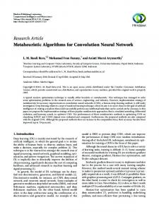
Start

E11

E12

E21

E22

…

…

W1

EN1

W2

…

WM ENM

EN2

Fig. 1: Illustration of the ants’ search space.

an ant decides which edge to take from Wk−1 to Wk , the pseudo random proportional rule given in Equation 3 is used.  α β arg maxi∈{1,...,N } (τik ηik ) q ≤ q0 i= (3) s otherwise. Here, α and β are parameters specifying the importance of pheromone and heuristic information, respectively. Moreover, q0 is a threshold and q ∈ U [0, 1], while s is an index selected probabilistically as:

4.2 Ant colony optimization ACO was originally proposed in [12]. An inspiring source of the ACO metaheuristic is the behavior of real ants searching for food. In short, ants make use of a chemical substance called pheromone, which is deposited on the ground. Initially, ants tend to wander around randomly in their search for food. If an ant finds food, it starts laying down trails of pheromone along its path back to the colony. If other ants find a path with pheromone, there is a high probability that the ants will stop wander randomly and instead follow the pheromone trail to the food source. Upon finding the food, they return to their colony, strengthening the pheromone trail. Pheromone however evaporates over time, and unless the trail is reinforced by any ants, it will eventually disappear. In terms of metaheuristic search, this decreases the probability of getting stuck in local optima. Using this behavior, ants are successful in cooperatively finding short(est) paths between their colony and food sources. There is a lot of different versions within the ACO framework, but we have used the ant colony system (ACS) suggested in [13]. According to [14], ACS is one of the best performing versions of ACO. Our implementation of ACS builds upon [8] and [7]. In the implemented algorithm, we create a number of ants that start out in the ant colony. From the colony, N edges lead to node W1 . From W1 , N edges lead to node W2 , etc., ending in the “food node” WM . Hence, the edge Eik taken from Wk−1 to Wk represents the target Ti to which weapon Wk should be allocated, and so, the complete path taken by an ant corresponds to a feasible solution to the static target-based WTA problem (see Figure 1). In an initialization phase, heuristic information ηik is assigned to each edge Eik according to the product Vi ×Pik , so that edges with higher products get a higher initial heuristic value (improving their chances of being selected). Initial pheromone τik is assigned uniformly to each edge, based upon a greedy shortest path heuristic (MMR). When

E1M E2M

Ps = P

α β τsk ηsk

α β l∈{1,...,N } τlk ηlk

.

(4)

That is, the target Ti to which weapon Wk should be allocated is greedily selected to be the target (edge) maximizing the product of the pheromone and heuristic information, given that q ≤ q0 . Otherwise, the target is determined through roulette wheel selection, where the amount of pheromone and heuristic information determines the probability for a target (edge) to be selected. When an ant reaches a new node (i.e., a weapon has been allocated to a target Ti ), it updates its local target values as Vi = Vi × (1 − Pik )Xik (where Xik = 1 if edge Eik has been used), affecting the ant’s heuristic information regarding the remaining edges, so that it becomes less likely that more weapons are assigned to the selected target in the ant’s generated solution. When the ant reaches the food node WM , the heuristic information is reinitialized, and a local update of pheromone is applied on the recently used edge as: τik = (1 − ϕ)τik + ϕτ0 ,

(5)

where ϕ ∈ [0, 1] is a constant regulating the pheromone evaporation. This local update is used for diversifying the paths taken by ants within the same iteration. After all ants within an iteration have reached WM , a global pheromone update is performed according to Equation 6, in which best ρ ∈ [0, 1] and ∆τik = 1/F best if edge Eik is part of the iteration-best solution, and 0 otherwise. best τik = (1 − ρ)τik + ρ∆τik .

(6)

In this way, the level of pheromone is increased for the path taken by the iteration-best ant, increasing the likelihood for this path to be taken by ants in future iterations. The global best solution is all the time kept track of, so that when no time remains, the best solution found during the search time is returned by the algorithm.

4.3 Particle swarm optimization

5. Experiments and results

PSO was originally introduced in [15]. The original version of PSO was intended for optimization problems with continuous decision variables, where each particle represents a candidate solution to the underlying problem at hand. Inspiration to PSO comes from the behavior of bird flocking [15]. Like birds, the particles move in a space, in which each particle pj in every time step t has an associated position x~j t and velocity v~j t . Together, the particles form a so called swarm. A particle’s position x~j t and velocity v~j t are in our case M -dimensional, i.e., each dimension represents a defensive weapon Wk . As an example, a particle having the position [2, 3, 2] indicates that we have a problem with three weapons, where the allocation suggests that W1 should be allocated to T2 , W2 to T3 , and W3 to T2 . Each particle is also t associated with a memory b~j storing the particle’s personal best position. Moreover, we also store the swarm’s global best position in the vector ~g t . In the initialization phase, each particle gets an initial position x~j 0 and velocity v~j 0 . The elements in the initial position vectors are integers randomly distributed between 1 and N , while the elements in the initial velocity vectors are real numbers randomly distributed from U [−N, N ]. The position and velocity for each particle is in our implementation of PSO updated according to Equation 7 and 8.

In the experiments reported here, we have used the open source testbed SWARD, running on a computer with a 2.4GHz Intel Core Duo CPU and 3GB RAM. We have tested different parameter settings, but the following setup has been used in the experiments, since they have shown to yield good results. For ACO, we have set nrOf Ants = max (N, M ), q0 = 0.5, α = 1, β = 1, ϕ = 0.1, and ρ = 0.1. For GA, nrOf Individuals = max (N, M ). Finally, for PSO, nrOf P articles = 50, c1 = 2.0, c2 = 2.0, and ω = 0.8. In addition to the three metaheuristic implementations, we have also included the well-known MMR algorithm and an algorithm based on random search for benchmarking purposes. The random search algorithm randomly generates feasible solutions as fast as possible, as long as there is time left. When no more time remains, the algorithm returns the best allocation found so far. The MMR algorithm works sequentially by greedily allocating weapons to the target maximizing the reduction of the expected target value. It starts with allocating the first weapon to the target for which the reduction in value is maximal, whereupon the value of the target is reduced to the new expected value. Once the first weapon is allocated, the same procedure is repeated for the second weapon, and so on, until all weapons have been allocated to targets. All the algorithms have been allowed to run for 2 seconds on each problem instance, which can be seen as a reasonable estimate of the time allowed for weapon allocation in a real-world air defense environment. In a second experiment, we have let the algorithms run for 60 seconds and plotted the quality of the solutions produced as a function of time, in order to investigate how much the performance of the algorithms are affected by the very tight real-time requirements in the first experiment.

t

v~j t+1 = ω v~j t + c1 r~1 t ◦ (b~j − x~j t ) + c2 r~2 t ◦ (~g t − x~j t ) (7) x~j t+1 = x~j t + v~j t+1

(8)

In Equation 7, ω is a parameter referred to as inertia or momentum weight, specifying the importance of the previous velocity vector. c1 and c2 are positive constants specifying how much a particle should be affected by the personal best and global best positions. These constants are often referred to as the cognitive and social components, respectively. r~1 t and r~2 t are vectors with random numbers drawn uniformly from [0, 1]. Moreover, the ◦operator denotes the Hadamard product, i.e., element-byelement multiplication of the vectors. After the position update specified in Equation 8, we round off the particles’ positions to their closest integer counterpart (since we can not have fractional assignments of weapons to targets). This is in accordance to how standard PSO is adapted to integer programming problems in [16]. Another problem that must be handled is what to do when particles move outside the bounds of the search space. When this happens, we reinitialize the position and velocity values of the coordinate for which the problem occurred. Moreover, in order to avoid premature convergence to local optima, we reinitialize the position and velocity vectors for particles rediscovering the current best solution.

5.1 Problem instance generation We have tested the algorithms on nine different problem sizes ranging from (N = 10, M = 10) up to (N = 30, M = 30). For each tested problem size, we have generated ten problem instances which have been averaged over when computing the results presented in Section 5.2. The problem instances have been generated in the open source testbed SWARD, in order to make it possible for other researchers to repeat the experiments presented here, and to test other algorithms on the same problem instances. The problem instances consist of randomly generated target values Vi ∈ U [25, 100] and kill probabilities Pik ∈ U [0.6, 0.9]. The reason for using these intervals is that they have been used in earlier research on SWTA, e.g., in [5]. In order to recreate an experiment with the same problem instances in SWARD, the parameters startN rOf T argets, startN rOf W eapons, stepN rOf T argets, stepN rOf W eapons, and nrOf Iterations should be set to 10, while

endN rOf T argets, and endN rOf W eapons are set to 30. The initial seed should be assigned the value 0.

5.2 Experimental results In Table 1-3, we show the mean objective function values returned by the algorithms after two seconds, averaged over 10 problem instances, together with the calculated standard deviations within parentheses. Due to the problem complexity, the quality of the produced solutions cannot in general be compared to the optimal solution, but for the (N = 10, M = 10)-problem instances, these have been identified by exhaustive search (which took several days to compute). The algorithms’ offset from the optimal average objective function value for that problem size are shown in the offset column in Table 1. Table 1: Mean F -values for N = 10. GA ACO PSO Random MMR

10 × 10 91.3 (9.8) 85.5 (7.9) 84.4 (7.4) 104.8 (7.7) 127.0 (11.8)

Offset 10.4% 3.4% 2.1% 26.8% 53.6%

10 × 20 15.4 (2.9) 15.0 (2.4) 12.5 (2.7) 24.7 (3.8) 25.2 (6.5)

10 × 30 2.4 (0.2) 2.6 (0.4) 2.2 (0.5) 5.2 (0.6) 5.1 (1.2)

Table 2: Mean F -values for N = 20. GA ACO PSO Random MMR

20 × 10 598.9 (82.6) 584.5 (83.5) 586.6 (84.0) 645.3 (77.9) 609.3 (72.5)

20 × 20 225.8 (17.6) 201.7 (17.2) 259.9 (38.4) 305.2 (28.9) 228.2 (24.4)

20 × 30 99.3 (6.8) 92.8 (6.4) 143.6 (10.8) 154.9 (13.4) 103.8 (14.0)

Table 3: Mean F -values for N = 30. GA ACO PSO Random MMR

30 × 10 1109.9 (64.4) 1098.5 (64.1) 1108.7 (56.0) 1179.7 (70.1) 1110.6 (63.6)

30 × 20 646.5 (59.6) 611.1 (52.5) 744.5 (56.2) 787.1 (72.5) 621.4 (47.9)

30 × 30 371.4 (34.4) 325.9 (30.2) 526.3 (66.0) 543.8 (59.7) 319.1 (27.1)

As can be seen, all the implemented metaheuristics are on average better than random search on all the tested problem sizes. ACO performs very well, since its produced solutions have the best average objective function value, or are close to the best average objective function value, on all problem sizes. The behavior of GA is stable, since the quality of its produced solutions is much closer to the best solutions than to the worst solutions on all problem sizes. The quality of the solutions produced by the PSO algorithm seems to be much more related to problem size. For small problem sizes its average objective function values are in the top, while they for larger problem sizes are much closer to the worst algorithm than to the best algorithm. The quality of the solutions produced by the random search algorithm and the MMR algorithm can be seen as baselines to which

the metaheuristics are compared. The performance of the random search algorithm is worse than the performance of the proposed metaheuristic algorithms on all problem sizes. The MMR algorithm is outperformed by the metaheuristic algorithms on all the small problem sizes where N = 10, but as the problem size (and thereby the solution space) increases, the solution quality of the fast MMR algorithm becomes better and better compared to the other algorithms, and actually is the best by far for the largest tested problem size (N = 30, M = 30). Hence, the utility of using evolutionary algorithms decreases with an increasing solution space, which is not surprising due to the tight real-time requirements. For getting a clearer picture of how the implemented algorithms perform in relation to each other, we have also calculated an average rank for the algorithms. This average rank information is presented in Figure 2. Looking at the average ranks, presented in Figure 2, we can see that the analysis of the results presented in Table 1-3 is strengthened. The average rank for the random search algorithm is higher than the corresponding rank for GA, ACO, and PSO, for all the tested problem sizes. The trend for the MMR algorithm is clear. Its average rank is the worst of all algorithms for the small problem sizes where N = 10, but the rank becomes better and better with an increasing solution space. This indicates that the implemented metaheuristic algorithms have problems to quickly produce high-quality solutions for large problem sizes. This is especially true for the PSO algorithm, which has the best rank for more small-scale problems, but only is better than random search for larger-scale problems. The stability of the GA algorithm is confirmed in Figure 2, but especially, the average rank of the ACO algorithms is worth noticing, which never becomes worse than 2.5, and is the best for 5 out of the 9 tested problem sizes. In order to investigate how the algorithms are affected by the tight real-time requirements used in the first experiment, we have in a second experiment let the algorithms run for 60 seconds each, on the ten problem instances of size (N = 20, M = 20) used in the first experiment. In Figure 3, we have plotted the quality of the best solution found by each algorithm with five second intervals for one of the problem instances. For the GA, it takes approximately 25 seconds to produce a solution with as good quality as the greedy MMR algorithm on this problem instance. This goes much faster for ACO and PSO, which both quickly produce better solutions than MMR. PSO is in this experiment the algorithm producing the best solution, which is a very different result from when the search time was limited to two seconds. The solution quality is heavily improved for PSO when allowed to search for a longer time, in this case with 33.3%.

6. Possible improvements From the results described in Section 5, it is clear that PSO gives good results for small problem instances, but

5 4,5 4

Average rank

3,5 3

GA ACO PSO Random MMR

2,5 2 1,5 1 0,5 0 10*10

10*20

10*30

20*10

20*20

20*30

30*10

30*20

30*30

Problem size

Fig. 2: Average rank (where 1.0 is the best possible and 5.0 is worst possible rank).

400

350

300

F-value

GA ACO PSO Random MMR

250

200

150 0

5

10

15

20

25

30

35

40

45

50

55

Time (s)

Fig. 3: F-value as a function of time when algorithms are run for 60 seconds on a problem instance of size (N = 20, M = 20).

Table 4: Mean F -values for (N = 20, M = 20). GA ACO PSO Random MMR

20 × 20 (2 s) 225.8 (17.6) 201.7 (17.2) 259.9 (38.4) 305.2 (28.9) 228.2 (24.4)

20 × 20 (60 s) 207.3 (21.1) 183.8 (19.2) 173.4 (19.0) 273.8 (30.2) 228.2 (24.4)

Improvement 8.2% 8.9% 33.3% 10.3% 0.0%

that the quality of the solutions is heavily decreasing with an increasing number of available weapon resources. A possible explanation for this might be that the particle swarm is likely to be searching in a few limited subparts of the search space due to the large impact of the current global best position. We have however tested with using a lower value of the social component c2 , without being able to increase the performance. Another reason might be that we for nrOf P articles use a fixed value, while the corresponding values for the other algorithms are set dynamically based upon the problem size. However, it is not clear how the number of particles should depend upon the size of the problem instance. In the implementations of PSO and GA, we have created individuals (particles and chromosomes) randomly from uniform distributions. Since the time available for search is very limited, it can make sense to seed some of the individuals in the initial generation using fast greedy heuristics such as the MMR algorithm. We think that this can be a suitable way to improve the performance of these two algorithms.

7. Conclusions We have described the target-based SWTA problem. Solving this problem in real-time is important for proper air defense, wherefore we have implemented three natureinspired metaheuristic algorithms adapted for SWTA into the testbed SWARD: ACO, GA, and PSO. We have in SWARD generated a set of problem instances of various size for evaluation. Each algorithm has been allowed to run for 2 seconds per problem instance, and the presented results have been averaged over ten problem instances. We have also let the same set of algorithms run for 60 seconds, in order to get an understanding for how much the real-time requirements affect the results. From the results obtained from the experiments, it is clear that the three suggested metaheuristics described in this paper perform better than random search on problem sizes between (N = 10, M = 10) and (N = 30, M = 30). It also seems clear that ACO is the metaheuristic algorithm with best real-time performance on problem instances with 20 or more targets. For the smallest problem instances, PSO give good results quickly, but the quality of the solutions produced by PSO becomes much worse as the number of weapon resources increases. Hence, PSO needs more time to produce solutions of high quality for problems with large search spaces. The quick and greedy MMR algorithm

is outperformed by the metaheuristic algorithms on small problem sizes, but as the search space increases, the quality of the solutions produced by MMR becomes better compared to the other algorithms. In fact, for the largest tested problem size, the MMR algorithm produces better real-time solutions than all the others. This indicates that greedy algorithms are more suitable than evolutionary algorithms for large problem sizes when there are tight real-time requirements.

Acknowledgment This work was supported by the Information Fusion Research Program (University of Skövde, Sweden) in partnership with Saab Electronic Defense Systems and the Swedish Knowledge Foundation under grant 2003/0104.

References [1] P. A. Hosein, “A class of dynamic nonlinear resource allocation problems,” Ph.D. dissertation, Massachusetts Institute of Technology, Dept. of Electrical Engineering and Computer Science, 1990. [2] F. Johansson and G. Falkman, “A Bayesian network approach to threat evaluation with application to an air defense scenario,” in Proceedings of the 11th International Conference on Information Fusion, 2008. [3] S. Lloyd and H. S. Witsenhausen, “Weapon allocation is NPcomplete,” in Proceedings of the 1986 Summer Conference on Simulation, 1986. [4] C. Huaiping, L. Jingxu, C. Yingwu, and W. Hao, “Survey of the research on dynamic weapon-target assignment problem,” Journal of Systems Engineering and Electronics, vol. 17, no. 3, pp. 559–565, 2006. [5] R. Ahuja, A. Kumar, K. Jha, and J. Orlin, “Exact and heuristic methods for the weapon target assignment problem,” Operations Research, vol. 55, no. 6, pp. 1136–1146, 2007. [6] G. G. den Broeder, R. E. Ellison, and L. Emerling, “On optimum target assignments,” Operations Research, vol. 7, no. 3, pp. 322–326, 1959. [7] Z.-J. Lee, C.-Y. Lee, and S.-F. Su, “Parallel ant colonies with heuristics applied to weapon-target assignment problems,” in Proceedings of the 7th Conference on Artificial Intelligence and Applications, 2002. [8] Z.-J. Lee, C.-Y. Lee, and S. F. Su, “An immunity-based ant colony optimization algorithm for solving weapon-target assignment problem,” Applied Soft Computing, vol. 2, pp. 39–47, 2002. [9] Z. J. Lee and W. L. Lee, “A hybrid search algorithm of ant colony optimization and genetic algorithm applied to weapon-target assignment problems,” in Proceedings of the 4th International Conference on Intelligent Data Engineering and Automated Learning, 2003. [10] X. Zeng, Y. Zhu, L. Nan, K. Hu, B. Niu, and X. He, “Solving weapon-target assignment problem using discrete particle swarm optimization,” in Proceedings of the 6th World Congress on Intelligent Control and Automation, 2006. [11] J. H. Holland, Adaptation in natural and artificial systems. University of Michigan Press, 1975. [12] M. Dorigo, “Optimization, learning and natural algorithms (in italian),” Ph.D. dissertation, Politecnico di Milano, 1992. [13] M. Dorigo and L. M. Gambardella, “Ant colony system: A cooperative learning approach to the traveling salesman problem,” IEEE Transactions on Evolutionary Computation, vol. 1, no. 1, pp. 53–66, 1997. [14] C. Blum and A. Roli, “Metaheuristics in combinatorial optimization,” ACM Computing Surveys, vol. 35, no. 3, pp. 268–308, 2003. [15] J. Kennedy and R. Eberhart, “Particle swarm optimization,” in Proceedings of IEEE International Conference on Neural Networks, 1995, pp. 1942–1948. [16] E. C. Laskari, K. E. Parsopoulos, and M. N. Vrahatis, “Particle swarm optimization for integer programming,” in Proceedings of the 2002 Congress on Evolutionary Computation, 2002.